COURSE CONTENT:
- Course Overview
- Week 1 - Control Structures
- Week 2 - Simulations
- PROJECT: Build Your Own R Package
- Week 3 - Regular Expressions
- Week 4 - Text Analysis
- Week 5 - GitHub Pages
- Week 6 - Data APIs
- Week 7 - Customized Reporting
Course Overview
CPP 527 is the second course in the Foundations of Data Science sequence.
This semester is designed to extend your working knowledge of data programming by introducing programming topics that will make you a more adaptive and creative analyst.
This course will cover:
- control structures like loops
- new data structures like lists
- regular expressions for working with text
- creation of packages in R
- creating of websites in GitHub
- building RMD templates to automate reporting
We will also cover the foundations of document design using both GitHub pages (free websites like this one) and customized RMD templates to enable you to better structure results from analytical projects.
The skills you learn this term can be used to build simulations in R, codify common workflows, and create specialized applications.
Course Cadence
The class is designed around labs each week and practice problems that you will discuss with classmates on YellowDig.
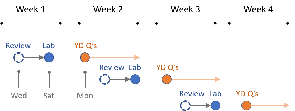
I will schedule review sessions early in the week so that you have a chance to start the new lab and come with questions.
You can post to YellowDig and participate in discussions throughout the week. I would request that you refrain from posting solutions to each week’s questions until Monday, though, so that everyone has a chance to share solutions. You can discuss the problems throughout the week.
There are three additional projects you must complete throughout the term. They are small projects, but require more autonomy than labs. Keep an eye out for these deadlines.
- Building an R package from code you develop on Labs 01-02 (due mid term)
- Build a report template (due end of term)
- Create a code-through tutorial (due end of term)
Getting Help
Note that similar to other courses the discussion board is run through the GitHub issues feature. It is a great forum tool because:
- You can format code and math using standard markdown syntax.
- You can cut and paste images directly into the message.
- You can direction responses using @username mentions.
Please use the discussion boards to practice your social coding etiquette.
- Ask clear questions.
- Provide sufficient code for the reader to diagnose the problem.
- When possible, use reproducible examples.
- Preview your responses before posting to ensure proper formatting.
Recall that you format code by placing fences around the code:
```
# your code here
lm( y ~ x1 + x2 )
```
The fences are three back-ticks. These look like quotation marks, but are actually the character at the top left of your keyboard (if you have a US or European keyboard).
GitHub does not have a native math rendering language (RMD documents, on the other hand, support formulas).
You have two options when using formulas: type them as regular text and use code formatting to make them clear (this option is usually sufficient).
```
y = b0 + b1•X1 + b2•X2 + e

b1 = cov(x,y) / var(x)
```
Or type your formula in a formula editor and copy and paste an image.
Use dput() to share R objects in a format that can be copied from the forum and pasted into R to recreate the vectors or data frames.
Practice Problem Warmup
Post on Monday, Aug 24th
Note that these are non-obvious bugs that can EASILY work there way into your code. Once you see the problem, it will seem obvious. But until you see it the code often looks fine and it’s unclear why it is not working as expected.
These practice problems are largely an opportunity to review content from CPP 526 and develop a sensitivity for the importance of writing robust and sustainable code, and testing your code for unexpected behaviors.
Many of these questions are similar to riddles or brain teasers that help sharpen your critical thinking skills when working with code. Work through them on your own, then discuss your ideas on YellowDig with classmates.
For the topics this week, you will find that reviewing the lecture notes on one-dimensional data types useful: VECTORS IN R.
Explain the following unexpected behaviors:
Q1: When is 5 larger than 10?
> (1:10) > 5
 [1] FALSE FALSE FALSE FALSE FALSE  TRUE  TRUE  TRUE  TRUE  TRUE
> (1:10) > "5"
 [1] FALSE FALSE FALSE FALSE FALSE  TRUE  TRUE  TRUE  TRUE FALSE
Q2: Invisible Dogs
x is a factor cataloging animals in a shelter, recording the type of animal.
Why can’t I count dogs?
> x  # TYPE OF ANIMAL (FACTOR)
[1] cat   dog   mouse
Levels: cat dog  mouse

> x == "cat"
[1]  TRUE FALSE FALSE
> x == "dog"
[1] FALSE FALSE FALSE
> x == "mouse"
[1] FALSE FALSE  TRUE
Q3: Average Years of Edu
I have a sample of 10 people and am trying to determine their average level of education. 12= high school degree, 16 = four-year college degree, etc.
My data is stored as a factor (which it should be since it is a categorical variable. But that makes it hard to calculate averages.
What is going wrong here?
grade.levels <- factor( c(12, 16, 12, 7, 7, 5, 6, 5, 9, 10) )

> # want to know average level of
> # schooling for sample:
> mean( grade.levels )
[1] NA
Warning message:
In mean.default(grade.levels) :
  argument is not numeric or logical: returning NA
>
> # mean requires a numeric variable
> mean( as.numeric( grade.levels ) )
[1] 3.8
Q4: String Sorting and Alphabetilization in R
Note that just as we compare numbers using greater-than, less-than, and equal-to operators, we can also compare strings.
Greater-than means that something occurs further along in the alphabet.
"b" > "a"
[1] TRUE
"a" > "b"
[1] FALSE
> "b" == "a"
[1] FALSE
Strings (words) that begin with identical letters are compared using subsequent letters:
"adam" > "abram"
[1] TRUE
When there is a tie capitalization also matters:
"A" > "a"
[1] TRUE
"a" > "A"
[1] FALSE
> "A" == "a"
[1] FALSE

"Aaron" > "aaron"
[1] TRUE
"aaron" > "Aaron"
[1] FALSE

"b" > "a"
[1] TRUE
> "b" > "A"
[1] TRUE
Considering these rules above, what will the following statement return?
"Aaron" > "abram"
And what does this tell us about how alphabetization occurs using logical operators?
Post your ideas to YellowDig
Week 1 - Control Structures
Unit Overview
Description
This section introduces control structures that will allow you to incorporate decision-making into computer code. It enables things like if-then logic to determine what code should be used based upon whether specified conditions are met.
Learning Objectives
Once you have completed this unit you will be able to:
- divide or “factor” your code into distinct tasks
- use functions as steps in problem-solving
- review compound statements
- implement if-else statements
- identify “edge cases” and their impact on code
Readings
Functions
Revisit the following chapter from last semester:
Make sure you are clear about:
- Arguments
- Object assignment (arrow) versus argument assignment (equals)
- When are quotation marks needed around arguments?
- Single-value arguments (one number or string) versus compound arguments (use
c()or pass existing objects) - Argument defaults
- Explicit and implicit use of argument names and positions
- Return values in R
- Function scope
Logical Statements
Recall that logical operators like EQUALS, NOT EQUAL, AND, OR, and OPPOSITE are used identify sets of cases that belong to a desired group, and sets of cases outside of the desired group.
==    EQUALS
!=    NOT EQUAL
&     AND
|     OR
!     OPPOSITE
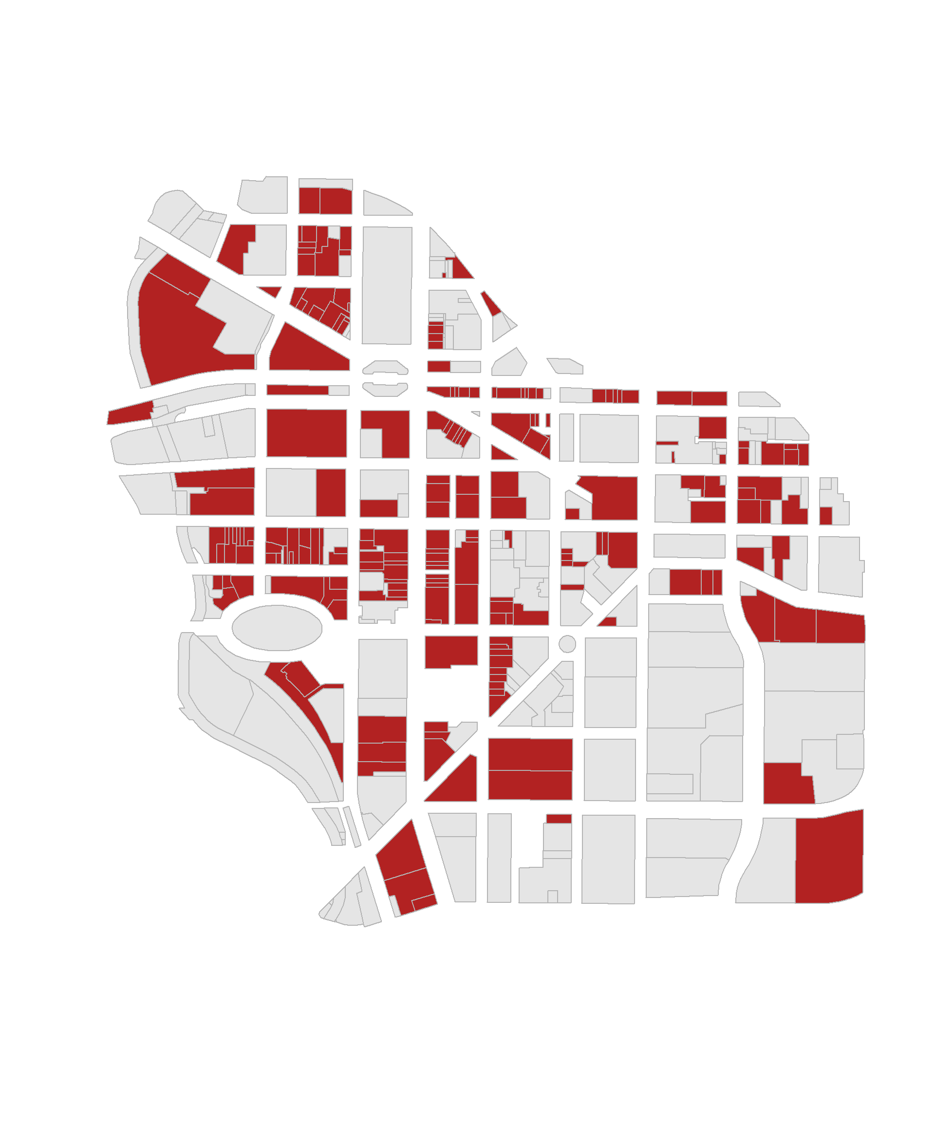
Recall that logical statements are used to construct groups. Group membership is encoded into logical vectors, where TRUE indicates membership and FALSE indicates cases that do not belong to the group. For example, identifying commercial properties in downtown Syracuse:
these <- downtown$landuse == "Commercial"
group.colors <- ifelse( these, "firebrick", "gray90" )
plot( downtown,  border="gray70", col=group.colors )
Compound logical statements require combining multiple criteria to define a group:
study.group == "TREATMENT" & gender == "FEMALE"
If you need a refresher, review the chapter on LOGICAL STATEMENTS.
Control Structures
Control structures are functions that allow you to implement logic or process in your code. They structure and implement the rules which govern our world. For example:
# pseudocode example
IF
  the ATM password is correct
  check whether the requested amount is smaller than account balance
  IF
    account balance > requested amount
    return requested amount
The most frequent control structures do the following:
- Only implement code if certain requirements are met (if-then or if-else functions)
- Implement code as long as a requirement is met (while loops)
- Repeat the same code for each item in a set (for loops)
Skim the following chapters for an introduction to a varietiy of control structures in R:
Quick Reference on Control Structures
In this lab we will focus on IF-THEN statements.
Next week we will introduce FOR LOOPS in order to build a simulation.
Scope
Many people are familiar with the expression “What happens in Las Vegas stays in Vegas.”
Scope is the rule that “what happens inside of functions stays inside of functions”.
It is very common to use variables like X or dat to represent objects in R. If you have defined a variable called X, and a different object called X is defined inside of a function you just called, how does R manage the conflict of having two objects X active at the same time?
Scope prevents actions inside of a function from impacting your active work environment.
For example, why is X not altered here except through assignment?
x <- 10

two.plus.two <- function()
{
  x <- 2 + 2
  return( x )
}

two.plus.two()
# [1] 4
x
# [1] 10

x <- two.plus.two()
x
# [1] 4
Note that the function two.plus.two() returns the object x, but after calling the function it does not replace the object x=10 that is active in the main environment. The function is returning values held by the variable x, but not exporting the object x itself.
In order to replace the X that is active in the environment, you need to assign the function results to the object.
x <- "iNiGo MoNtoyA"

fix_names <- function( x )
{
  x <- toupper( x )
  return( x )
}

fix_names( x )
# [1] "INIGO MONTOYA"
x
# [1] "iNiGo MoNtoyA"

x <- fix_names( x )
x
# [1] "INIGO MONTOYA"
You need to be familiar with the general concept of scope (what happens inside functions stays inside functions), but only at a superficial level for now.
For more details see: Scoping Rules of R.
Planning Your Code with Pseudo-Code
Typically as you start a specific task in programming there are two things to consider.
(1) What are the steps needed to complete the task? (2) How do I implement each step? How do I translate them into the appropriate functions and syntax?
It will save you a huge amount of time if you separate these tasks. First, take a step back from the problem that think about the steps. Write down each step in order. Make some notes about what data is needed from the previous step, and what the return result will be from the current step.
Think back to the cooking example. If we are going to bake cookies our pseudo-code would look something like this:
- Preheat the oven.
- In a large bowl, mix butter with the sugars until well-combined.
- Stir in vanilla and egg until incorporated.
- Addflour, baking soda, and salt.
- Stir in chocolate chips.
- Bake.
Note that it lacks many necessary details. How much of each ingredient? What temperature does the oven need to be? How long do we bake for?
Once we have the big picture down and are comfortable with the process then we can start to fill in these details:
- Preheat the oven.
- Preheat to 375 degrees
- In a large bowl, mix butter with the sugars until well-combined.
- 1/3 cup butter
- 1/2 cup sugar
- 1/4 cup brown sugar
- mix until the consistency of wet sand
Note that in computer programming terms butter, sugar, and brown sugar are the inputs or arguments needed for a function. The wet sand mixture is the return value of the process.
In the final step, we will begin to implement code.
# 1. Preheat the oven.
#    - preheat to 375 degrees

preheat_oven <- function( temp=375 )
{
   start_oven( temp )
   return( NULL )
}


# 2. In a large bowl, mix butter with the sugars until well-combined.
#    - 1/3 cup butter
#    - 1/2 cup sugar
#    - 1/4 cup brown sugar
#    - mix until the consistency of wet sand

mix_sugar <- function( butter=0.33, sugar=0.5, brown.sugar=0.25 )
{
   sugar.mixture <- mix( butter, sugar, brown.sugar )
   return( sugar.mixture )
}


# 3. Stir in vanilla and egg until incorporated.
#    - add to sugar mixture
#    - mix until consistency of jelly

add_wet_ingredients <- function( sugar=sugar.mixture, eggs=2, vanilla=2 )
{
   # note that the results from the previous step are the inputs into this step
}
We are describing here the process of writing pseudo-code. It it the practice of:
- Breaking an analytical task into discrete steps.
- Noting the inputs and logic needed at each step.
- Implementing code last.
Pseudo-code helps you start the process and work incrementally. It is important because the part of your brain that does general problem-solving (creating the basic recipe) is different than the part that drafts specific syntax in a langauge and de-bugs the code. If you jump right into the code it is easy to get lost or derailed.
More importantly, pseudo-code captures the problem logic, and thus it is independet of any specific computer language. When collaborating on projects one person might generate the system logic, and another might implement. So it is important to practice developing a general overview of your task at hand.
Here are some helpful examples:
Lab-01 - Control Structures
Due Saturday, August 29th
This lab is based upon the famous Monty Hall Problem.
Although there was much debate about the correct solution when it was initially introduced there are many concise explanations of the proper solution:
Using Computing Logic to Build the Game
The Monty Hall Problem is a great example of a mathematical problem that might be hard to solve using proofs, but it is fairly easy to solve using simulation.
Since it is a game with simple and explicit rules we can build our own virtual version. Then we can compare how outcomes differ when we deploy the two different strategies for selecting doors.
In Lab 01 we will use control structures to build a virtual version of the game. In Lab 02 we will use simulation to play the game thousands of times so that we can get stable estimates of the payoff of each strategy.
Submit Solutions to Canvas:
YellowDig Practice Problems
Post on Monday, Aug 31st
UPDATE TO INSTRUCTIONS: Please post your solution to ONE of the questions below on YellowDig (Q1-A and Q1-B each count as one question).
This gives you a chance to explain your solution a little more clearly and it minimizes duplicate solutions on the discussion board.
See what has been posted already before deciding which solution you will post.
You can then discuss solutions to problems you did not post on other pins posted by classmates. Comment if you see problems with the proposed solutions or possible alternative solutions.
Q1: FACTORS
Q1-A: Ordering Levels
By default factors created in R will order levels (categories) alphabetically.
In many cases levels have a meaningful order other than alphabetization.
For example, days of the week, months of the year, etc.
How can you alter this factor so that it correctly orders the days of the week?
x <- c("MON","TUE","WED","THUR","FRI","SAT","SUN")
vec <- sample( x, 100, replace=TRUE )
f <- factor( vec )
table( f )

f
 FRI  MON  SAT  SUN THUR  TUE  WED
  14   18   14    9   16   16   13
Side note: in R the term levels describes categories in a categorical variables (a factor).
In regression, we use the term levels to describe numerical dosages of a treatment, such as milligrams of caffeine in a heart rate study.
In regression, the term factor is also used synonymously with explanatory variable or covariate. For example, what other factors might explain elevated heart rates in patients? Age could be one factor, race could be another factor. In this context factor is a cause, not a categorical variable.
Make a mental note that factor and level are both precise technical terms that have different meanings in computer science and statistics.
Q1-B: Empty Levels
How can we drop empty levels from a factor?
f2 <- f[ f %in% c("MON","TUE","WED","THUR","FRI") ]
table( f2 )
Q1-C: Counting Zeros
What about cases where counts of zeros are important? What if we wanted to note here days that events did not occur?
Create a new factor that will report levels that do not occur in a sample.
x <- c("TUE","WED","FRI","SUN")
vec <- sample( x, 20, replace=TRUE )
f3 <- factor( vec )
table( f3 )
Q2: COMPARISON OF SETS
Recall the structure of IF STATEMENTS:
if( logical statement )
{  code that only executes if TRUE }
It’s important to note that the logical statement must return a SINGLE T/F value. If you use a logical vector as the argument in the IF condition then it will use the first T/F values in the vector and ignore the rest (which is problematic in many instances).
The logical EQUALS operator == compares elements in two vectors in order. It will return the same number of T/F as length(x).
If you want to test whether two vectors are the same use the identical() function, which always returns a single T/F value:
x <- c("A","B","C")
y <- c("A","B","C")

x == y
[1] TRUE TRUE TRUE
identical( x, y )
[1] TRUE

# incorrect
if( x == y )
{  some code  }

# correct
if( identical( x, y ) )
{  some code  }
Q2-A: Ignore Order
Perhaps you want to run a chunk of code only IF two vectors contain the same elements, but order is irrelevant.
Note that in most cases X and Y will represent vectors of observations. The order and position of vectors is extremely important. Changing the order or a vector will corrupt the data.
x <- c("tom","nancy","sara")
y <- c("male","female","female")
d <- data.frame( name=x, gender=y )
In this case X and Y represents sets of elements, so the positions are not important.
Update this case to compare the two sets X and Y to see if they contain the same elements while ignoring order.
x <- c("A","B","C")
y <- c("B","A","C")

identical( x, y )
[1] FALSE
Q2-B: Ignore Vector Length
Similar to the case above, we want to compare these two sets to ensure they contain the same elements. We don’t care about how many times each element occurs, just that the two sets are the same.
How can we ignore the number of elements here?
x <- c("A","B","A","C")
y <- c("B","C","B","A","C")

identical( x, y )
[1] FALSE
Q2-C: Data Types
This is an interesting case because the logical operator == will consider these vectors to be identical, but the identical() function will not.
x <- c(1,2,3)
y <- c("1","2","3")

x == y
[1] TRUE TRUE TRUE
identical( x, y )
[1] FALSE
The reason for this is that logical operators will implicitly cast data types in order to compare two objects that have different data types. You saw this last week:
5 > 10
[1] FALSE

# implicitly casts both as character vectors
5 > "10"
[1] TRUE
How would you adapt the code here so it compares the two vectors and ignores the data type.
x <- c(1,2,3)
y <- c("1","2","3")
identical( x, y )
Does you solution also work with this example?
x <- c(01,02,03)
y <- c("01","02","03")
Q2-D: Comparisons with Missing Values
Missing values are important in statistics and data analytics, but they pose some challenges for computer logic.
Note the behavior of logical operations here:
# missing info for both individuals
x <- c("A",NA,"C")
y <- c("A",NA,"C")

x == y
[1] TRUE    NA  TRUE
identical( x, y )
[1] TRUE

# missing info for one individual
x <- c("A","B","C")
y <- c("A",NA,"C")

x == y
[1] TRUE    NA  TRUE
identical( x, y )
[1] FALSE
Write a statement that compares two vectors while ignoring missing cases.
Does your code also work with the following cases?
x <- c("A","A","B",NA,"C","C")
y <- c("A",NA,"B","B","C","C")
x <- c("A","A","B","B","C","C")
y <- c("A",NA,"B",NA,"C","C")
Q3: ROUNDING ERRORS
This is one of the most unexpected and somewhat shocking errors you can encounter in computer science:
x <- 0.5 - 0.3
y <- 0.3 - 0.1

x
[1] 0.2
y
[1] 0.2


x == y
[1] FALSE
# FALSE on most machines

identical( x, y )
[1] FALSE
To see what is happening here print the difference of the variables:
x - y
[1] 2.775558e-17
It turns out that numbers with decimals are hard to represent in computer memory, so very tiny rounding errors can be introduced in calculations. They are not noticed unless the numbers are compared at the smallest scale.
# 1.051
# 1.052
1.1 equals 1.1
1.05 equals 1.05
1.051  does NOT equal  1.052
In the example above the variables X and Y are identical up until the 17th decimal point.
The tiny difference was introduced by converting decimal numbers to their binary representation as a string of 0’a and 1’s in ther computer’s memory while doing the mathematical calculations behind the scenes.
This tiny tiny rounding error will tyically only pose a problem in logical statements. And only if the conversion introduces a rounding error, which is typically not the case:
x <- 5 - 3
y <- 3 - 1
x == y
[1] TRUE

x <- 0.1 + 0.1
y <- 0.0 + 0.2
x
[1] 0.2
y
[1] 0.2
x == y
[1] TRUE
The formal and robust solution is to use the all.equal() function when comparing numerical objects.
USE THIS APPROACH IN YOUR CODE.
x <- 0.5 - 0.3
y <- 0.3 - 0.1
all.equal( x, y )
[1] TRUE
Explain why these also work:
x <- 0.5 - 0.3
y <- 0.3 - 0.1

x2 <- round( x, 1 )
y2 <- round( y, 1 )

x2
[1] 0.2
y2
[1] 0.2

x2 == y2
[1] TRUE

x3 <- as.character( x )
y3 <- as.character( y )

x3
[1] "0.2"
y3
[1] "0.2"

x3 == y3
[1] TRUE
Q4: APPROXIMATE MATCHES
In this example vectors represent sets of traits of pairs of individuals in a study.
- race (white/minority)
- gender (male/female)
- college degree? (college/highschool)
We want to identify people that are similar but not necessarily identical.
Create a function that compares the two individuals and returns TRUE if they are the same on at least two traits, and false if they only match on one or zero traits.
compare_pairs <- function( x, y )
{
   # your code here
}


x1 <- c("white","female","college")
y1 <- c("white","female","college")
compare_pairs( x1, y1 )
# SHOULD BE TRUE

x2 <- c("minority","female","college")
y2 <- c("white","female","college")
compare_pairs( x2, y2 )
# SHOULD BE TRUE

x3 <- c("minority","female","college")
y3 <- c("white","male","college")
compare_pairs( x3, y3 )
# SHOULD BE FALSE

x4 <- c("minotity","female","college")
y4 <- c("white","male","high school")
compare_pairs( x4, y4 )
# SHOULD BE FALSE
CHALLENGE QUESTION
Q5: COUNTING SUBSTRINGS
In all of the examples above we were comparing two things.
# is it a nine?
x <- c( 1, 9, 10, 19, 99, 09 )
x == 9
[1] FALSE  TRUE FALSE FALSE FALSE  TRUE
Recall that logical statements can be used to count things.
# is it a nine?
x <- c( 1, 9, 10, 19, 99, 09 )
sum( x == 9 )
[1] 2
Q5-A: How would you count all nine’s in the vector?
For example, 19 contains one nine, 99 contains two nines.
Q5-B: How would you count all of the elements of X that CONTAIN a nine?
For example, 19 contains a nine.
Q5-C: Count all 17’s in the vector X.
X is a vector containing the numbers 1 to 1,000.
x <- 1:1000
How can you count the number of times “17” occurs in the vector?
For example, the number 117 contains a 17. The number 170 also contains a 17.
Week 2 - Simulations
Unit Overview
Description
This section introduces loops. We will use them to create simulations.
Learning Objectives
Once you have completed this section you will be able to
- use a loop responsibly in your code
- select appropriate iterators
- be mindful of the collector vector needed for the loop
Assigned Reading
Required:
Building Simulations in R: Mastering Loops
Creating Animations with Loops
Recommended: these readings are a slightly more advanced treatment of loops and control structures used in simulations. Dive in or bookmark them for later.
Examples of loops used to create effective data visualization:
Why Americans Are So Damn Unhealthy, In 4 Shocking Charts
LOOP EXAMPLE
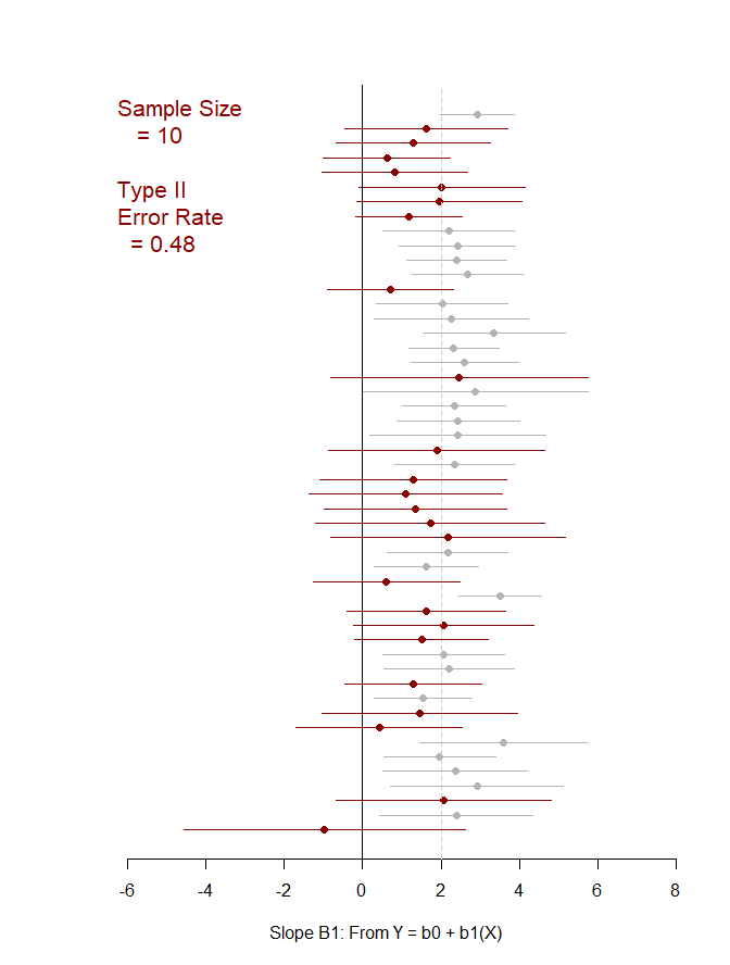
This example demonstrates the use of loops to create a simulation to examine the how model statistics might vary for a given sampling framework.
In this case we are taking repeated random draws of size N from a population, then calculating the slope and confidence interval of the slope. We want to note cases where b1 contains zero since these would represent NULL results in our study.
These types of bootstrapping simulations are very useful for generating robust versions of sampling statistics when the data is irregular or closed-form solutions do not exist.
In this case were are interested in statistical power as a function of sample size. In studies like drug trials it might cost $10,000 for each study participant, so drug companies want to minimize the sample size needed to veryify the effectiveness of their drugs.
We can use previous research to ascertain a reasonable correlation between X and Y or anticipated effect size to simulate some population data.
Type II Errors represent cases that the regression fails to produce a slope that is differentiable from zero (the confidence interval of slope b1 contains zero).
We would start with a small sample size (n=10 in this example) then increase it until we have exceeded a target Type II Error rate.
Some helper functions were created to generate the proper statistics inside of the loops.
Pay attention to differences in the constructors.
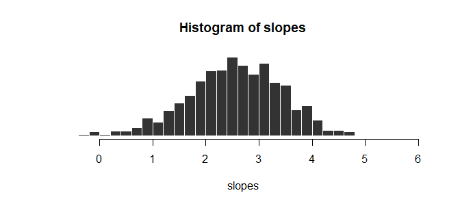
The first example collects only the slope from each simulation, so results are stored in a collector vector called slopes.
# BOOTSTRAPPING TYPE II ERRORS
# Examine Type II Errors
# as a function of sample size

# load data and helper functions
source( "https://raw.githubusercontent.com/DS4PS/cpp-527-fall-2020/master/lectures/loop-example.R" )
head( d )                       # data frame with X and Y
get_sample_slope( d, n=10 )     # returns a single value
test_for_null_slope( d, n=10 )  # returns a one-row data frame

## EXAMINE SLOPES
## sample size = 10


slopes <- NULL  # collector vector

for( i in 1:1000 )  # iterator i
{

  b1 <- get_sample_slope( d, n=10 )
  slopes[ i ] <- b1

}


# descriptives from 10,000 random draws, sample size 10

head( slopes )
[1] 2.246041 3.979462 1.714822 4.689032 1.763237 3.107451

summary( slopes )
#    Min. 1st Qu.  Median    Mean 3rd Qu.    Max.
#  -2.194   1.596   2.176   2.088   2.600   4.868

=======
summary( slopes )
#    Min. 1st Qu.  Median    Mean 3rd Qu.    Max.
#  -2.194   1.596   2.176   2.088   2.600   4.868

>>>>>>> Stashed changes
hist( slopes, breaks=25, col="gray20", border="white" )
The second example generates the slope, confidence interval (lower and upper bounds), and a null significance test from each new sample. The results are stored in a data frame called results.
## EXAMINE CONFIDENCE INTERVALS
## sample size = 10

# build the
# results data frame
# using row binding


results <- NULL

for( i in 1:50 )
{

  null.slope.test <- test_for_null_slope( d, n=10 )
  results <- rbind( results, null.slope.test )

}


head( results )

# confidence intervals from 50 draws, sample size 10

#            b1 ci.b1.lower ci.b1.upper null.slope
# x  -0.9783359  -4.5757086    2.619037       TRUE
# x1  2.3897431   0.4295063    4.349980      FALSE
# x2  2.0781628  -0.6677106    4.824036       TRUE
# x3  2.9178206   0.7080918    5.127549      FALSE
# x4  2.3702949   0.5238930    4.216697      FALSE
# x5  1.9701996   0.5513491    3.389050      FALSE

plot_ci( df=results )
## alternative constructor:
## the list version
## runs faster but it
## needs to be converted
## to a data frame afterwards

results <- list()

for( i in 1:50 )
{

  null.slope.test <- test_for_null_slope( d, n=10 )
  results[[ i ]] <- null.slope.test

}

## convert list to df
results <- dplyr::bind_rows( results )

head( results )
plot_ci( df=results )
Lab 02
Due Saturday, September 5th
This lab uses material from the simulation slides:
Building Simulations in R: Mastering Loops
Submit Solutions to Canvas:
YellowDig Practice Problems
Post on Monday, Sept 7th
Q1 - GAMBLING STREAKS AND DURATION MODELS
We covered a very basic animation in the lecture notes - a random walk.
Start game with $10 in cash. At each step you flip a coin and win a dollar, lose a dollar, or stay the same.
How long does it take for a player to lose all of their money?
While loops are useful when we repeat a process until a condition is met, the player being out of money in this case.
cash <- 10
results <- NULL
count <- 1
while( cash > 0 )
{
  cash <- cash +
    sample( c(-1,0,1), size=1 )
  results[count] <- cash
  count <- count + 1
}
Q1-A: Visualize the Game
Similar to the lecture notes, create a visualization of the cash that a player has at each round of the game until they go broke.
Q1-B: You’ve got to know when to fold them
Starting with $10 in the game, how long does it take the typical player to go bankrupt?
If you don’t want to do a complicated mathematical proof, create a simulation, play the game 10,000 times, then report the average duration of each game.
Side note, would the mean or the median be a better measure of the average here?
I would suggest wrapping the code above into a play_game() function and calling that function repeatedly inside your loop.
Note: the interesting edge case in this simulation is a case where a person never goes broke so your program runs forever.
Is this a likely outcome when the players all start with $10?
How would you adapt your code to account for this scenario?
Q1-C: Finding Warren Buffet
If you run a simulation of 10,000 individuals playing the game, all starting with $10, how many individuals will never go broke?
Operationalize never in your code and explain your assumptions.
How many of these individuals did you find in your simulation?
Q2 - ANIMATIONS
A random walk is a one-dimensional outcome (cash in hand) tracked over time.
Physicists have used a similar model to examine particle movement with a Brownian Motion model.
It is similar to the betting model above except for each time period the particle moves in two dimensions.
x <- 0
y <- 0
for( i in 1:1000 )
{
  x[i+1] <- x[i] + rnorm(1)
  y[i+1] <- y[i] + rnorm(1)
}
Q2-A: Create the Brownian Motion animation above
Use the loop above to generate particle positions.
Create an animation to visualize the movement of the particle.
Discuss the package or app you used to generate the GIF.
Q2-B: Shadow of the past
If animations move too quickly it will look like popcorn and it can be hard to identify the meaningful patterns in the data.
You can enhance the information value of animations by visualizing change and in addition to the current model state include information on past stages.
How would you create the trailing tail in this animation?
Q2-C: Alternative Animations
If you are not interested in Brownian Motion, share another animation you can create using loops.
Discuss the package or app you used to generate the GIF.
Share your ideas with classmates on YellowDig:
PROJECT: Build Your Own R Package
Due Saturday, September 19th
Building Packages in R
At some point you might develop a tool that you want to upload to the CRAN so it is widely available.
More likely, if you are working with a team of analysts within an organization you will begin building a library of functions that are specific to the project.
Even if not sharing the package widely it is often a more efficient method for the team to maintain project code so that it can be easily updated and functions enhanced. Project updates are then easily shared simply by re-installing the package.
This tutorial will teach you how to build and share a package in R. You will “package” your R code from Labs 01 and 02 into a new montyhall package to make it easier to run simulations to evaluate game strategies.
Instructions
Submit to Canvas:
To receive credit for the assignment, submit the URL to your package on GitHub.
Grading:
Your package will be installed and submitted to a series of testing scripts that ensure each function operates as expected.
The documentation will also be inspected to ensure there are complete instructions and sample code available for each of the functions.
You will receive a grade of zero if you package cannot be installed or run, and you will lose 5 points if documentation is unavailable.
Week 3 - Regular Expressions
Unit Overview
Text as Data:
So this week comes with an up-front warning. You can get a PhD in Natural Language Processing, which is an entire field devote to computation tools used to process and analyze text as data. We have one week to cover the topic!
We obviously cannot go too deep into this interesting field, but let’s at least motivate some of the R functionality with a couple of cool examples.
Which Hip-Hop Artist Has the Largest Vocabulary?
Who is the Anonymous Op-Ed Writer inside the Trump Administration?
These examples all demonstrate interesting uses of text as data. They are also examples of the types of insight that can come from analysis with big data - the patterns are hiding in plain sight but our brains cannot hold enough information at one time to see it. Once we can find a system to extract hidden patterns from language we can go beyond seeking large public databases to generate insights, and we can start using all of Twitter, all published news stories, or all of the internet to identify trends and detect outliers.
Required Reading
String Processing & Regular Expressions:
The core of all text analysis requires two sets of skills. Text is computer science is referred to as “strings”, a reference to the fact that spoken languages mean nothing to computers so they just treat them as strings of letters (words) or strings of words (sentences). String processing refers to a set of functions and conventions that are used to manipulate text as data. If you think about the data steps for regular data, we clean combine, transform, and merge data inside of data frames. Similarly there are operations for important text datasets (often lots of documents full of words), cleaning them (removing words, fixing spelling errors), merging documents, etc. Core R contains many string processing functions, and there are lots of great packages.
“Regular expression” are a set of functions used to aid in processing text by defining very precise ways to query a text database by looking for specific strings, or more often strings that match some specific pattern that has meaning. For example, if I gave you the following text with everything but punctuation replaced by X, you could still tell me what the word are for:
- xxxxx@xxx.com (email address)
- www.xxxxxxxx.xxx (web URL)
- @xxxxxxx (social media handle)
So regular expressions can be very useful for searching large databases for general classes of text, or alternatively for searching for generic text that occurs only in a very specific context (at the beginning or end of a word, in the middle of a phrase, etc.).
Helpful Reference Material:
Lab-03: Regular Expressions
Due Saturday, September 12th
Instructions
Submit Solutions to Canvas:
YellowDig Practice Problems
Post on Monday, Sept 14th
WARM-UP:
The function grep( pattern, string ) works as follows:
Search for the pattern in each of the strings in the character vector at the top, strings.
The search pattern in each case below represents a regular expression.
What will the following cases return?
strings <- c("through","rough","thorough","throw","though","true","threw","thought","thru","trough")

# what will the following return?

grep( pattern="th?rough", strings, value = TRUE)

grep( pattern=".ough", strings, value = TRUE)

grep( pattern="^.ough", strings, value = TRUE)

grep( pattern="ough.", strings, value = TRUE)

grep( pattern="[^r]ough", strings, value = TRUE)

# these are not as useful

grep( pattern="tr*", strings, value = TRUE)

grep( pattern="t*o", strings, value = TRUE)
Q1 - Constructing Factors
Building on the lab from this week, we constructed groups of titles using the following code logic:
group.questions <- grepl( "//?$", titles )

# OR

group.who <- grepl( "^Who", titles )
group.what <- grepl( "^What", titles )
group.where <- grepl( "^Where", titles )

group.www <- group.who | group.what | group.where
What if we wanted to build a single factor that has distinct levels for all of our groups? Note that you would need to define MUTUALLY EXCLUSIVE groups in order for this to make sense. If the groups are not mutually exclusive (one title could belong to multiple groups) then it would not make sense to combine them into a single factor.
group.01 <- grepl( ..., titles )  # questions
group.02 <- grepl( ..., titles )  # colons
group.03 <- grepl( ..., titles )  # power lists

# create factor f where each level represents a different kind of title
# and include an "other" category for those that don't fit into above groups
Q2: RegEx Substring Application
We have an large database where all of the addresses and geographic coordinates are stored as follows:
x <- c("100 LANGDON ST
MADISON, WI
(43.07794869500003, -89.39083342499998)", "00 N STOUGHTON RD E WASHINGTON AVE
MADISON, WI
(43.072951239000076, -89.38668964199996)")
Write a function that accepts the address vector x as the input, and returns a vector of numeric coordinates.
Note that the length of addresses can change, so you will need to use regular expressions (instead of just a substr() function) to generate proper results.
Week 4 - Text Analysis
Unit Overview
This week will use regular expressions you developed during the prior week and some additional text analysis tools from the package quanteda to practice working with text as data.
Required Reading
Review some of the examples from last week in order to see content analysis (counts and pattens of words) and sentiment analysis in practice:
Which Hip-Hop Artist Has the Largest Vocabulary?
Who is the Anonymous Op-Ed Writer inside the Trump Administration?
Quanteda
There are several text analysis packages in R, but Quanteda is one of the most popular and robust.
Text analysis packages contain functions that assist in the manipulation of text as data in order to convert raw text files into structured databases, apply a variety of pre-processing steps that clean and standardize the data, and functions that assist in identifying patterns in text.
Read the Quanteda Quick-start Guide to familiarize your self with some basic components of text analysis.
Focus on:
- Vocabulary:
- Document: a file consisting primarily of text
- Corpus: a collection of documents in a study
- Tokens: single words or phrases
- Cleaning text:
- Removing punctuation and often numbers and symbols
- Pre-Processing Steps:
- Stemming words to remove variant components: running, runner, runs -> run
- Identify proper nouns
- Combine compound words into single words: George Bush -> george_bush
- Analysis
- Tokenization of pre-processed documents
- Identification of patterns in use of words
Lab-04 - Text Analysis
Due Saturday, September 19th
Submit Solutions to Canvas:
YellowDig Practice Problems
Post on Monday, Sept 21st
This week’s YellowDig component is a little different. You are asked to read some recent work looking at the crisis of reproducibility in research, and some possible explanations for low reproducibility in specific fields.
The Crisis of Scientific Reproducibility
The topic this week is an introduction to the hugely important topic of reproducibility in science, the ability to reproduce results from ground-breaking scientific work that was published in top journals. For a long-time there was an assumption that peer-review meant that each scientist subjected their work to fellow scientists that were experts on their topic, and thus it provides a solid barrier to error-prone and work from being published.
The notion of reproducibility, however, grew from fields like physics and chemistry where early lab experiments could be described with enough precision for another scientist to mix the same chemicals, or recreate the same conditions for a gravity experiment, and easily verify whether the claims in the paper were defensible.
Things get a lot more complicated now that (1) the data requirements necessary to publish in top journals have expanded, (2) methods have become much more complicated, and (3) science is very competitive with high-stakes rewards for winning grants or covetted endowed professor positions, resulting in proprietary data, data collection techniques, or lab conditions like stem cell lines or bacteria strains that cannot be easily replicated. As a result, peer reviewers have to take a lot of what authors say on face value without having enough information to challenge certain assertions, or without having access to the raw data and thousands of lines of code that produces the results that are being defended in the paper. Furthermore, weaknesses in how statistical methods are reported have introduced systematic bias into the types of research that gets published in top journals (it has to be splashy, and thus more likely to be anomoly studies than reproducible work).
If you are not going into academics, should you care? Yes, because the problems with reproducibility in science are just a proxy for problems with data analysis that will arise in any organization outside of academics as well. Scientists experience pressure to publish. Consultants also experience pressure to do work fast, and to identify patterns that will impress clients. These sorts of issues will arise in any environment where data brings value. In science we care about making the process transparent so that others can replicate work. If you are a manager or project lead for a team of analysts, you should care about transparency because it allows you to ensure your team is doing the job correctly, especially if your name is going on the report!
This week’s topic introduces you to the fascinating topic of the replication crisis in science. Your task will be to read two articles on reproduciblity in science:
When the Revolution Came for Amy Cuddy, New York Times Magazine, 2017
How Quality Control Could Save Science
You are welcome to skim additional articles on the topic conveniently catalogued by Nature Magazine:
Challenges in irreproducible research
For the discussion topic this week, I would like you to argue either:
(1) that the reproducibiilty crisis can be effectively ended if science adopts new technologies and better practices, or
(2) that the problems with reproducibility are so engrained in the limits of science and in the DNA of academic institutions that there will always be problems with reproducility, and attempts to address it are insufficient in their ability to get to the root of the problem, or naive about human nature.
Pick a side and make your case!
Week 5 - GitHub Pages
Unit Overview
A big part of every analysts job is trying to find ways to distill large volumes of data and information down to meaningful bites of knowledge, often for diverse stakeholder audiences that have varying degrees of technical expertise. For this reason, communication skills are extremely valuable for data scientists. You will constantly be challenged to find the interesting story that emerges from an overwhelming amount of data, and find creative ways to tell the story so that information becomes actionable.
Although it might not sound as edgy as building a machine learning classifier, the ability to create customized reporting formats and automate various steps of analysis will both make you more efficient and also more effective at communication.
This lab introduces you to one powerful tool for your toolkit - using GitHub pages to build a website quickly and inexpensively (for free, actually). Then use it to host various components of projects including public-facing reports and RMD documents after rendering.
For the project component of the course we will use a CV template to learn how the pagedown package can be used to create highly-customized report templates:
We will also practice automation by the separation of the design elements of reporting from the data contained in the reports. In this example for a CV, Nick Strayer’s positions are stored in a CSV file on GitHub:
And they are added to the document templates using some custom functions which filter positions and loop through the list to iteratively build the document.
```{r}
print_section(position_data, 'education')
```
These are accomplished with text formatting functions that are a little more advanced than where you are at now. But if you are curious, they are basically just taking lists of text, putting it into tables, and formatting the tables. The formatting functions are HERE.
GitHub Pages Set-Up
This week’s lab will ask you to configure a GitHub page within a repository on your account. GitHub pages are an amazing resource because (1) they allow you to create an unlimited number of websites related to your projects FOR FREE, and (2) they can be created and maintained using Markdown, which simplifies a lot of the complexity of websites. You will learn to link HTML files generated from R Studio so that you can start sharing analytical projects with external audiences.
The set-up of a simple GitHub page is fairly straight-forward and can be completed in a few basic steps:
This will give you a barebones website with a landing page you can write using Markdown, and a few templates that you can select from.
You have access to myriad advanced features on the platform. GitHub pages leverage several powerful web frameworks like Jekyll, Bootstrap, Liquid, and Javascript to make customization of static pages both easy and powerful. We will spend some time talking about how the pieces of a website fit together so that you have a rudimentary knowledge of the platform:
More importantly, GitHub pages can help demonstrate the concept of page templates. We can design the layout of a graphic, table, or section of text on a page then dynamically populate it with data. GitHub pages allow you to do with with basic HTML and Liquid tags:
And the pagedown package in R allows you to develop a variety of templates using similar principles:
Similar to other work we have done in R, we will start by using some working examples then reverse engineer them so you can see how the pieces fit together. You are not expected to master any of these topics in the short time-frame of the semester. The proper benchmark of knowledge is can you take an existing open source project and adapt it as necessary.
Cascading Style Sheets
You will not be required to learn web programming languages like HTML and Javascript (though they are super useful if you invest the time). You do, however, need to become familiar with very basic CSS as it is impossible to do customization without it. CSS started as a somewhat modest project but has evolved into a powerful language. R Markdown documents support CSS, which makes them fully customizable. It will also become more important so you begin to develop dashboards or custom interactive Shiny apps, since CSS is the primary means of controlling layouts and other style elements.
These two pages on the example GitHub site have the same content, but CSS elements are used to change the page layout and style on the second. Click on the “see page layout” button to see the CSS elements.
Required Reading
Skim the following chapters, reading to get a general sense of concepts and the basics of how each might function. You can skip sections that explain the code in detail. I am more concerned that you understand how these basic pieces fit together, and when you hear terms like “responsive” you conceptually know what people are talking about.
Introduction to Web Programming
Lab 05
Due Saturday, September 26th
Instructions for Creating a GitHub Page
The animation in the Unit Overview above shows how simple it is to activate GitHub pages for any project repository so that you can turn markdown files into web-hosted HTML files and share tutorials or reports created from RMD files.
If we want a website with a bit more functionality, however, we will need to start from an existing template and adapt it.
For this lab you will copy and then adapt an existing GitHub pages websites.
Start by forking the beautiful-jekyll website template:
Beautiful Jekyll Website Template on GitHub
Update:
The Beautiful Jekyll site has been adding new features and additional complexity. For this assignment it helps to start simple.
I would recommend cloning a simple site that was built using Beautiful Jekyll such as:
Note that forking a project on GitHub creates a copy of the project on your account. You can update files without impacting the originals. Forking a project retains the link back to the original project so that you can add updates from the original version and if desired send pull requests back to the original with code updates that improve their project (this is how contributions to open-source projects are made).
When you clone a site, you copy all of the files to your account (similar to forking), but you sever ties between the two projects. This is done if you want to take the code as it exists and then modify it to create a new project that is distinct from the original. It means you can’t incorporate updates from the original project and you can’t send suggested code updates back to the original project.
You fork a project when you want to continue to contribute back to the original or continue to incorporate updates made in the original project. You clone a repository if you want to take the code as it stands and adapt it as something new. You still need to attribute the original project after cloning, but there will be no formal link between the repositories on GitHub after cloning.
After forking or cloning a site, follow the instructions in the README file to begin customizing your page.
In the _config.yml file in the default directory do the following:
Change the website name and description.
# Name of website
title: My website

# Short description of your site
description: A virtual proof that I'm awesome
You can update social network IDs if you like, or replace Dean’s info with empty quotes "" so the social media icons are present but not active.
Change the color scheme for the website:
# Personalize the colors in your website. Colour values can be any valid CSS colour

navbar-col: "#F5F5F5"
navbar-text-col: "#404040"
navbar-children-col: "#F5F5F5"
page-col: "#FFFFFF"
link-col: "#008AFF"
hover-col: "#0085A1"
footer-col: "#F5F5F5"
footer-text-col: "#777777"
footer-link-col: "#404040"
Add Page and Update Navigation
You have forked the master branch of the website, which does not include the “getting started” page on the live site menu:
Navigate to the getting started content located in the README.md file in the BeautifulJekyll repo, and copy the file content (the raw markdown text) to a new file called getstarted.md in the main folder on your site. Be sure to copy text from the raw view of the page with the markdown code and not the formatted version that does not include markdown tags.
Now update the navigation bar and add another option called “Getting Started” under “Resources”. You will use the text “getstarted” for the URL, excluding the .md markdown extension. GitHub pages converts all markdown files to HTML files in the background, so you want to direct the user to the HTML version, which does not require an explicit extension to work in browsers:
# List of links in the navigation bar
navbar-links:
  About Me: "aboutme"
  Resources:
    - Beautiful Jekyll: "http://deanattali.com/beautiful-jekyll/"
    - Learn markdown: "http://www.markdowntutorial.com/"
    - Getting Started: "getstarted"                         # ADD THIS LINK
  Author's home: "http://deanattali.com"
The index.html file contains text from the landing page of the website. You will find some page title and descriptions in the YAML header of this file:
---
layout: page
title: My website
subtitle: This is where I will tell my friends way too much about me
use-site-title: true
---
Change the Text Style on the Getting Started Page
Demonstrate that you are able to apply CSS styles to specific elements of a page.
Create a new div section around Step 1 on the Getting Started page.
### Overview of steps required

There are only three simple steps, ....

Here is a 40-second video ....

<img src="../img/install-steps.gif" style="width:100%;" alt="Installation steps" />


<div class="gs-section-01" markdown="1">


### 1. Fork the Beautiful Jekyll repository

Fork the [repository](https://github.com/daattali/beautiful-jekyll)
by clicking the Fork button on the top right corner in GitHub.


</div>
Note that in order to render markdown text between HTML <div> tags you need to do two things:
(1) Make sure your file is a markdown .md file type and not an HTML .html file.
Either will work with GitHub pages, but only the .md files are automatically converted from MD to HTML on the GitHub (kramdown) servers. If you add markdown elements to an HTML file type they will not be converted.
(2) Add a markdown=”1” attribute or double-squirrely brackets
By default any markdown that occurs between HTML div tags is not converted to HTML. To instruct the server-side parser to process the text as markdown you need to add the markdown=”1” attribute to the div tag, or wrap the markdown text in double-squirrely brackets.
Option 1:
<div class="gs-section-01" markdown="1">

### 1. Fork the Beautiful Jekyll repository

Fork the [repository](https://github.com/daattali/beautiful-jekyll)
by clicking the Fork button on the top right corner in GitHub.

</div>
Option 2:
<div class="gs-section-01">


{{

### 1. Fork the Beautiful Jekyll repository

Fork the [repository](https://github.com/daattali/beautiful-jekyll)
by clicking the Fork button on the top right corner in GitHub.

}}


</div>
Follow the Barebones Jekyll example for customizing a page style by adding a CSS style sheet the bottom of the Getting Started page:
<style>

.gs-section-01 h3 {
     color: red }

.gs-section-01 p {
     font-size: 30px;
}

</style>
Similarly, add new div sections around Step 02 and Step 03 on the page so that each step has different header styles and text. It doesn’t have to look nice - just show you are able to selectively change the style on a page.
Create a Liquid Table
Using the Barebones Jekyll Custom Table example add a page with a custom table.
Copy the liquid-table.html template and add it as a new layout in your site’s layout folder. You will need to change the parent page template on the liquid-table.html page to “default” or “page” in your new site (you don’t have a nice-text layout that you can use as the parent page layout).
---
layout: default
---
Create a new page in your main website folder called table-demo.md and copy the page content from the Barebones Jekyll example.
You will need to add the ryan-v-ryan.jpg image to your img folder for it to be accessible on your new site (you can right-click and save it, then drag it into the image folder on your GitHub site).
You do not need to include the “See Page Layout” button.
---
layout: liquid-table
title: 'amiright?'
reynolds:
strengths:
- good father
- funny
- dated alanis morissette
weaknesses:
- singing
- green lantern movie
- tennis backhand
gosling:
strengths:
- builds houses
- is a real boy
- never dated alanis morissette
weaknesses:
- micky mouse club
- cries a lot
- not ryan reynolds
---

### Lorem Ipsum
Lorem ipsum dolor sit amet....
Add the page to your navigation bar:
# List of links in the navigation bar
navbar-links:
  About Me: "aboutme"
  Resources:
    - Beautiful Jekyll: "http://deanattali.com/beautiful-jekyll/"
    - Learn markdown: "http://www.markdowntutorial.com/"
    - Getting Started: "getstarted"
  Table Demo: "table-demo"              # ADD THIS LINK
When these steps are done, submit a link to (1) your live site and (2) your GitHub repo where the website lives.
Submit Solutions to Canvas:
And share your page link on YellowDig:
YellowDig Practice Problems
Post on Monday, Sept 28th
TIDY DATA:
This exercises introduces the extremely important but simple concept of tidy data.
The development of tidy data has been driven by my experience working with real-world datasets. With few, if any, constraints on their organisation, such datasets are often constructed in bizarre ways. I have spent countless hours struggling to get such datasets organised in a way that makes data analysis possible, let alone easy. I have also struggled to impart these skills to my students so they could tackle real-world datasets on their own. In the course of these struggles I developed the reshape and reshape2 (Wickham 2007) packages. While I could intuitively use the tools and teach them through examples, I lacked the framework to make my intuition explicit. This paper provides that framework. It provides a comprehensive “philosophy of data”: one that underlies my work in the plyr (Wickham 2011) and ggplot2 (Wickham 2009) packages.
Tidy data is a standard way of mapping the meaning of a dataset to its structure. A dataset is messy or tidy depending on how rows, columns and tables are matched up with observations, variables and types.
In tidy data:
- Each variable forms a column.
- Each observation forms a row.
- Each type of observational unit forms a table.
The basic idea is that data should be selectable with code, so attributes should not be coded as row or column names. They should be represented as distinct variables.
This makes data exploration and manipulation feasible and efficient.
You have seen that there are many tidyverse functions (from the dplyr package especially) that replicate core R functions, but return tidy results instead of default formats:
table( dat$Gender_Drv1, dat$Gender_Drv2 )

          Female Male Unknown
  Female    4622 5463      85
  Male      5637 7707      96
  Unknown    776  835      25

dplyr::count( dat, Gender_Drv1, Gender_Drv2 )

  Gender_Drv1 Gender_Drv2    n
1      Female      Female 4622
2      Female        Male 5463
3      Female     Unknown   85
4        Male      Female 5637
5        Male        Male 7707
6        Male     Unknown   96
7     Unknown      Female  776
8     Unknown        Male  835
9     Unknown     Unknown   25
These two tables are equivalent, but in the second case we can do things like drill down further into the data by isolating accidents caused by male drivers (Driver 1), or we can color-code male and female data on a graph using a driver attribute with col=factor(Gender_Drv2).
In the default table version we can’t even get a range of group size since we can’t analyze table values easily (you can always re-convert the table object back to vectors and extract column and row attributes, but it takes some work).
When attributes are built into the table as row names and column names they can no longer be manipulated directly. This is the general idea of tidy data - retain all of the information and store it in a way that makes it useful for subsequent analysis.
In the tidyverse specifically, most analytical and graphical packages will assume that your data is in a tidy format as the default way to organize data. That is not true with older R packages.
The convention has gained traction, though, and there is a big movement toward using tidy data as the standard for data frames and function outputs in R. This makes work-flow much easier! Using pipes to create a data recipe, for example, is possible primarily because of tidy conventions.
To learn more, read pages 1-8 of the article that introduced this concept focusing on understand what a tidy dataset looks like (the examples of tidy versus non-tidy datasets are most useful). You can skim the remaining pages that discuss some advanced approaches to automate conversion from non-tidy to tidy formats. For now understanding the concept is more important than automation of conversion steps.
Practice the concept with the problems below:
Q1: Table Conversion
R contains some built-in datasets that consist of pre-tabulated data.
Convert one of the three sets of tables to a tidy dataset.
- Titanic
- HairEyeColor
- UCBAdmissions
Share the tidy dataset (not the code) on YellowDig.
Note that it is a conceptual exercise, not a programming exercise. The goal is to get the tidy table structure correct, not find a function that can automate the process (the paper presents some automation steps you can ignore for now).
You can do the exercise in Excel, or you can build vectors manually and combine them into a data frame. You just need to share the tidy table, not the process used to create it.
Titanic
, , Age = Child, Survived = No

      Sex
Class  Male Female
  1st     0      0
  2nd     0      0
  3rd    35     17
  Crew    0      0

, , Age = Adult, Survived = No

      Sex
Class  Male Female
  1st   118      4
  2nd   154     13
  3rd   387     89
  Crew  670      3

, , Age = Child, Survived = Yes

      Sex
Class  Male Female
  1st     5      1
  2nd    11     13
  3rd    13     14
  Crew    0      0

, , Age = Adult, Survived = Yes

      Sex
Class  Male Female
  1st    57    140
  2nd    14     80
  3rd    75     76
  Crew  192     20


HairEyeColor
, , Sex = Male

       Eye
Hair    Brown Blue Hazel Green
  Black    32   11    10     3
  Brown    53   50    25    15
  Red      10   10     7     7
  Blond     3   30     5     8

, , Sex = Female

       Eye
Hair    Brown Blue Hazel Green
  Black    36    9     5     2
  Brown    66   34    29    14
  Red      16    7     7     7
  Blond     4   64     5     8


UCBAdmissions
, , Dept = A

          Gender
Admit      Male Female
  Admitted  512     89
  Rejected  313     19

, , Dept = B

          Gender
Admit      Male Female
  Admitted  353     17
  Rejected  207      8

, , Dept = C

          Gender
Admit      Male Female
  Admitted  120    202
  Rejected  205    391

, , Dept = D

          Gender
Admit      Male Female
  Admitted  138    131
  Rejected  279    244

, , Dept = E

          Gender
Admit      Male Female
  Admitted   53     94
  Rejected  138    299

, , Dept = F

          Gender
Admit      Male Female
  Admitted   22     24
  Rejected  351    317
Q2: Dummy Variable Conversion
This data frame contains some outcome Y for observations in four states.
dat
   Y NY AL FL MN
1 54  1  0  0  0
2 27  1  0  0  0
3 35  0  1  0  0
4 19  0  1  0  0
5 99  0  0  1  0
6 84  0  0  1  0
7 34  0  0  0  1
8 29  0  0  0  1
The states are currently presented as dummy variables.
To make the dataset tidy convert the four dummy variables into a single STATE factor.
This problem should be done programmatically. There are several ways to do this effectively.
# dput( dat )
dat <-
structure(list(Y = c(54L, 27L, 35L, 19L, 99L, 84L, 34L, 29L),
    NY = c(1, 1, 0, 0, 0, 0, 0, 0), AL = c(0, 0, 1, 1, 0, 0,
    0, 0), FL = c(0, 0, 0, 0, 1, 1, 0, 0), MN = c(0, 0, 0, 0,
    0, 0, 1, 1)), class = "data.frame", row.names = c(NA, -8L
))
Bonus: after you have created a single STATE factor, identify a function that will re-convert the factor into dummy variables.
Challenge Question:
Convert this dplyr count table into a regular table format that can be included in a report.
d2
  Gender_Drv1 Gender_Drv2    n
1      Female      Female 4622
2      Female        Male 5463
3      Female     Unknown   85
4        Male      Female 5637
5        Male        Male 7707
6        Male     Unknown   96
7     Unknown      Female  776
8     Unknown        Male  835
9     Unknown     Unknown   25

d2 <-
structure(list(Gender_Drv1 = structure(c(1L, 1L, 1L, 2L, 2L,
2L, 3L, 3L, 3L), .Label = c("Female", "Male", "Unknown"), class = "factor"),
    Gender_Drv2 = structure(c(1L, 2L, 3L, 1L, 2L, 3L, 1L, 2L,
    3L), .Label = c("Female", "Male", "Unknown"), class = "factor"),
    n = c(4622L, 5463L, 85L, 5637L, 7707L, 96L, 776L, 835L, 25L
    )), row.names = c(NA, -9L), class = "data.frame")
Regular format:
          Female Male Unknown
  Female    4622 5463      85
  Male      5637 7707      96
  Unknown    776  835      25
Week 6 - Data APIs
Unit Overview
Introduction:
Nice Overview of APIs
Data journalists describe the value of APIs.
Example APIs:
There is one API that you likely use every single day: Google. Your query takes the form of the search words you type into the box, and the data is sent back as a nicely-formatted list of websites: the page title, URL, and the first few sentences of text on the page.
The Data Science Toolkit site has a lot of nice examples of these type of APIs in action.
These mostly have user interfaces where you paste some input data into a search box and it returns data based upon your inputs.
For example, you can type an address and it will return a set of latitude and longitude coordinates.
Alternatively, if you want to query news sources for stories on specific topics check out:
How do APIs Work?
APIs function like calls to a database. You send parameters, and the server sends the appropriate response - the data that matches your query.
The interface for many APIs functions a lot like a dplyr::filter call. You specify which slice of data you would like through the values you designate:
data %>%
  filter(  gender=="male"   &  age=="20-25"  &  state %in% c("AZ","NY","PA") )
The main difference is that this is a filter function manipulating data on your own computer. Data APIs allow you to query a database that lives on a server.
Data APIs consist of a base URL that serves as the address of the data on the server and a set of allowable queries.
Each API defines it’s own set of allowable queries. Similar to a filter() function there are rules about how to construct your statements so they identify the proper slice of data. Unlike R, if you violate the defined rules of the API then instead of an error you just get an empty set with no data.
For demonstration purposes, assume that we want to download some census data from a nice Graphical User Interface (GUI) someone has created for us in order to make the Census API easier to use. It might look something like this:
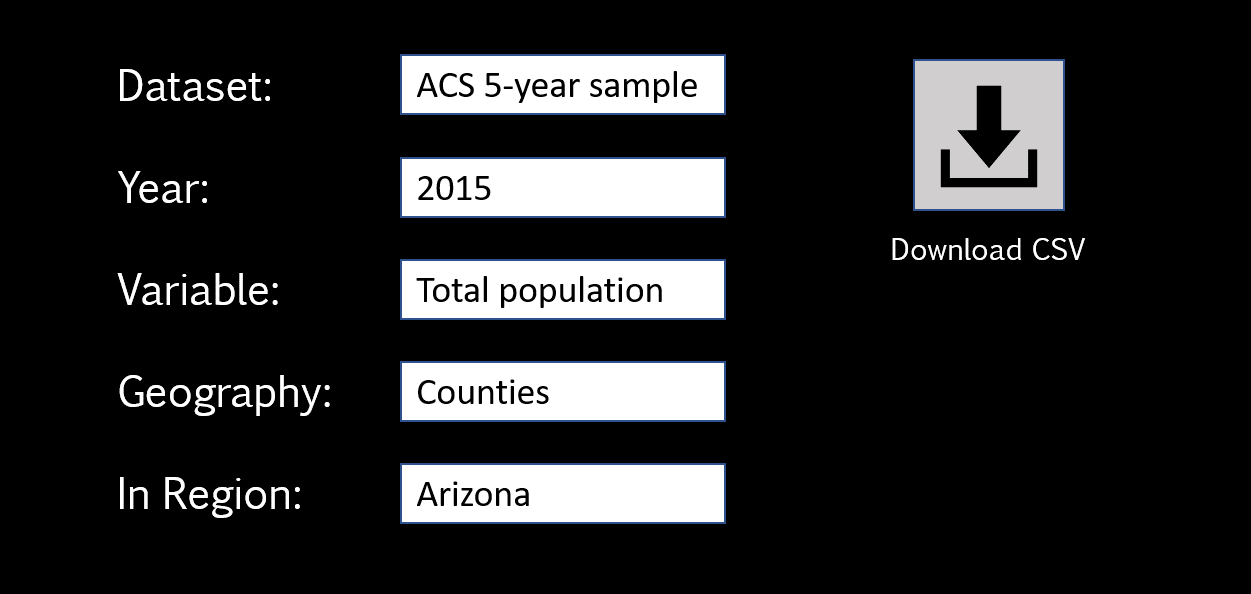
All we need to do is select options from drop-down lists and click “download” to receive all of the data as a CSV file.
APIs operate basically the same, but we would use the API documentation to convert the same query in this GUI into the API URL directly.
To run this example, you will need to get your own free Census API key and replace “your.unique.census.key.goes.here” with the actual key you receive from the Census.
I have selected the population variable B01001_001E but you can find other variable names in the Census catalog: https://api.census.gov/data/2015/acs/acs5/variables.html.
library( censusapi )
library( jsonlite )
library( httr )

##################################################################
####      API QUERY:
##################################################################

API.BASE     <- "https://api.census.gov/data"
API.VINTAGE  <- "2015"
API.NAME     <- "acs/acs5"
VARIABLE     <- "B01001_001E"      # TOTAL POPULATION (E for Estimate)
STATE        <- "04"               # AZ STATE FIPS CODE
KEY          <- "your.unique.census.key.goes.here"

##################################################################

BASE.URL <- paste( API.BASE, API.VINTAGE, API.NAME, sep="/" )
BASE.URL

# [1] "https://api.census.gov/data/2015/acs/acs5"

FULL.URL <- paste( BASE.URL, "?get=NAME,", VARIABLE, "&for=state:", STATE, "&key=", KEY, sep="" )
FULL.URL

# [1] "https://api.census.gov/data/2015/acs/acs5?get=NAME,B01001_001E&for=state:04&key=your.unique.census.key.goes.here"
Now, pasting this URL into a browser is the equivalent of sending a query to a database. Similar to the filter() function you are referencing variable names and specific values (logical statements) and separating them with an &:
?get=                  # start of the query
NAME,B01001_001E       # list of variable names
&
for=state:04           # geography
&
key=your.unique.census.key.goes.here
The data is returned in a JSON format:
[["NAME","B01001_001E","state"],
["Arizona","6641928","04"]]
That’s it! It’s that easy.
Just like functions in R, you will look up the API arguments in the documentation.
The documentation should also tell you the types of values that each argument expects. For example, the state geography uses FIPS codes (state:04) instead of the normal two-letter abbreviation (state:AZ).
In order to import the data into R we need a couple more steps.
- We need to retrieve the data from the API URL that we have built.
- We need to convert from JSON to a matrix, then the matrix to a data frame.
We can write a couple of functions to make this easier:
api.data.raw <- httr::GET( FULL.URL )

matrix_to_df <- function( m )
{
  d <- as.data.frame(m)
  col.names <- d[ 1, ]    # get first row
  names(d) <- col.names   # assign as column names
  d <- d[ -1 , ]          # delete first row
  return(d)
}


json_to_data_frame <- function( api.data.raw )
{
    data.as.json <- httr::content( api.data.raw, as = "text" )
    data.as.matrix <- jsonlite::fromJSON( data.as.json )
    data.as.df <- matrix_to_df( data.as.matrix )
    return( data.as.df )

}


json_to_data_frame( api.data.raw )  # returns a data frame
     NAME   B01001_001E   state
2 Arizona       6641928      04

# intermediate data formats for reference

data.as.json
[1] "[[\"NAME\",\"B01001_001E\",\"state\"],\n[\"Arizona\",\"6246816\",\"04\"]]"

data.as.matrix
     [,1]      [,2]          [,3]
[1,] "NAME"    "B01001_001E" "state"
[2,] "Arizona" "6246816"     "04"
Another example grabbing data from all of the states instead of one at a time:
KEY           <- "your.unique.census.key.goes.here"
API.BASE      <- "https://api.census.gov/data"
API.VINTAGE   <- "2015"
API.NAME      <- "acs/acs5"
VARIABLE      <- "B01001_001E"      # TOTAL POPULATION (E for Estimate)
STATE         <- "*"                # ALL STATES

BASE.URL <- paste( API.BASE, API.VINTAGE, API.NAME, sep="/" )
FULL.URL <- paste( BASE.URL, "?get=NAME,", VARIABLE, "&for=state:", STATE, "&key=", KEY, sep="" )

api.data.raw <- httr::GET( FULL.URL )

json_to_data_frame( api.data.raw )

                   NAME B01001_001E state
2               Alabama     4830620    01
3                Alaska      733375    02
4               Arizona     6641928    04
5              Arkansas     2958208    05
6            California    38421464    06
7              Colorado     5278906    08
8           Connecticut     3593222    09
9              Delaware      926454    10
...etc
You can drill down further and further depending upon the API options. For example to get the population of every county in the US we would use the following geography:
for=county:*&in=state:*
The Census API gets complicated quickly because there are several hundred datasets you can query, several dozen allowable geographies for each variable, and several thousand variables to choose from.
This is why packages like censusapi will include a bunch of functions that just list API options:
apis <- censusapi::listCensusApis()
head( apis[,1:3], 25 )
                                                                  title              name vintage
451                     Annual Economic Surveys: Annual Business Survey             abscb    2017
454                     Annual Economic Surveys: Annual Business Survey            abscbo    2017
458                     Annual Economic Surveys: Annual Business Survey             abscs    2017
391 American Community Survey: 1-Year Estimates: Detailed Tables 1-Year          acs/acs1    2005
395 American Community Survey: 1-Year Estimates: Detailed Tables 1-Year          acs/acs1    2006
397 American Community Survey: 1-Year Estimates: Detailed Tables 1-Year          acs/acs1    2007
399 American Community Survey: 1-Year Estimates: Detailed Tables 1-Year          acs/acs1    2008
403 American Community Survey: 1-Year Estimates: Detailed Tables 1-Year          acs/acs1    2009
71                                           ACS 1-Year Detailed Tables          acs/acs1    2010
86                                           ACS 1-Year Detailed Tables          acs/acs1    2011
97                                           ACS 1-Year Detailed Tables          acs/acs1    2012
179                                          ACS 1-Year Detailed Tables          acs/acs1    2013
202                                          ACS 1-Year Detailed Tables          acs/acs1    2014
243                                          ACS 1-Year Detailed Tables          acs/acs1    2015
265                                          ACS 1-Year Detailed Tables          acs/acs1    2016
288                                          ACS 1-Year Detailed Tables          acs/acs1    2017
365 American Community Survey: 1-Year Estimates: Detailed Tables 1-Year          acs/acs1    2018
501 American Community Survey: 1-Year Estimates: Detailed Tables 1-Year          acs/acs1    2019
72                                       ACS 1-Year Comparison Profiles acs/acs1/cprofile    2010
87                                       ACS 1-Year Comparison Profiles acs/acs1/cprofile    2011
100                                      ACS 1-Year Comparison Profiles acs/acs1/cprofile    2012
177                                      ACS 1-Year Comparison Profiles acs/acs1/cprofile    2013
204                                      ACS 1-Year Comparison Profiles acs/acs1/cprofile    2014
245                                      ACS 1-Year Comparison Profiles acs/acs1/cprofile    2015
266                                       ACS 1-Year Comparison Profile acs/acs1/cprofile    2016
In summary, this lecture introduces the basic concepts behind a data API.
You are doing this:
But manually by building your API query like this:
KEY           <- "your.unique.census.key.goes.here"
API.BASE      <- "https://api.census.gov/data"
API.VINTAGE   <- "2015"
API.NAME      <- "acs/acs5"
VARIABLE      <- "B01001_001E"      # TOTAL POPULATION (E for Estimate)
STATE         <- "04"               # AZ STATE FIPS CODE

BASE.URL <- paste( API.BASE, API.VINTAGE, API.NAME, sep="/" )
FULL.URL <- paste( BASE.URL, "?get=NAME,", VARIABLE, "&for=state:", STATE, "&key=", KEY, sep="" )
FULL.URL

# [1] "https://api.census.gov/data/2015/acs/acs5?get=NAME,B01001_001E&for=state:04&key=your.unique.census.key.goes.here"
Data APIs are often the fastest way to get data, but more importantly they also document the process used to acquire the data.
That makes the process easy to replicate later, and also easy to inspect if there are problems with the data.
The best part is that most useful APIs have already been turned into packages in R, so you don’t even need to read all of the documentation. You can download the package then use R functions directly. For example, the function for the Census API might look something like this:
get_census_data <- function( VINTAGE, API.NAME, VARIABLE, STATE, KEY )
{
   API.BASE <- "https://api.census.gov/data"
   BASE.URL <- paste( API.BASE, VINTAGE, API.NAME, sep="/" )
   FULL.URL <- paste( BASE.URL, "?get=NAME,", VARIABLE, "&for=state:", STATE, "&key=", KEY, sep="" )
   api.data.raw <- httr::GET( FULL.URL )
   df <- json_to_data_frame( api.data.raw )
   return( df )
}
If you are curious, you can view the source code for the censusapi package to see how the code is actually constructed. It is more complicated because it has to account for combinations of all of the different arguments using all of the APIs, along with error-checking. The devil is always in the details!
Additional Reading:
If you have an important dataset that you would like to share with the world, you can also build your own API in R:
Lab 06
Due Saturday, October 3rd
THIS LAB IS OPTIONAL
Scaling Your Analysis w Functions and Loops
If you recall from CPP 526 we discussed the example where Ben Balter, GitHub’s official government evangelist, created a project to make Washington DC open GIS files more accessible and useful by converting them all to a format more amenable to open-source projects (geoJSON files).
Ben wrote a script that downloaded all of Washington DC’s open data files, converted them to better formats, then uploaded them to GitHub so others have access:
https://github.com/benbalter/dc-maps
The geoJSON files can also be read into R directly from GitHub, making it easy to incorporate the spatial maps and data into a wide variety of projects:
library( geojsonio )
library( sp )
github <- "https://raw.githubusercontent.com/benbalter/dc-maps/master/maps/2006-traffic-volume.geojson"
traffic <- geojson_read( x=github, what="sp" )
plot( traffic, col="steelblue" )
Recall the lab where you created one Dorling cartogram for your neighborhood clustering project:

library( geojsonio )   # read shapefiles
library( sp )          # work with shapefiles
library( sf )          # work with shapefiles - simple features format
library( tmap )        # theme maps
library( dplyr )       # data wrangling
library( pander )      # nice tables


crosswalk <- "https://raw.githubusercontent.com/DS4PS/cpp-529-master/master/data/cbsatocountycrosswalk.csv"
crosswalk <- read.csv( crosswalk, stringsAsFactors=F, colClasses="character" )

# search for citie names by strings, use the ^ anchor for "begins with"
grep( "^MIN", crosswalk$msaname, value=TRUE )

# select all FIPS for Minneapolis
these.minneapolis <- crosswalk$msaname == "MINNEAPOLIS-ST. PAUL, MN-WI"
these.fips <- crosswalk$fipscounty[ these.minneapolis ]
these.fips <- na.omit( these.fips )

state.fips <- substr( these.fips, 1, 2 )
county.fips <- substr( these.fips, 3, 5 )

dat <- data.frame( name="MINNEAPOLIS-ST. PAUL, MN-WI",
                   state.fips, county.fips, fips=these.fips )
dat
| name | state.fips | county.fips | fips |
|---|---|---|---|
| MINNEAPOLIS-ST. PAUL, MN-WI | 27 | 003 | 27003 |
| MINNEAPOLIS-ST. PAUL, MN-WI | 27 | 019 | 27019 |
| MINNEAPOLIS-ST. PAUL, MN-WI | 27 | 025 | 27025 |
| MINNEAPOLIS-ST. PAUL, MN-WI | 27 | 037 | 27037 |
| MINNEAPOLIS-ST. PAUL, MN-WI | 27 | 053 | 27053 |
| MINNEAPOLIS-ST. PAUL, MN-WI | 27 | 059 | 27059 |
| MINNEAPOLIS-ST. PAUL, MN-WI | 27 | 123 | 27123 |
| MINNEAPOLIS-ST. PAUL, MN-WI | 27 | 139 | 27139 |
| MINNEAPOLIS-ST. PAUL, MN-WI | 27 | 141 | 27141 |
| MINNEAPOLIS-ST. PAUL, MN-WI | 27 | 163 | 27163 |
| MINNEAPOLIS-ST. PAUL, MN-WI | 27 | 171 | 27171 |
| MINNEAPOLIS-ST. PAUL, MN-WI | 55 | 093 | 55093 |
| MINNEAPOLIS-ST. PAUL, MN-WI | 55 | 109 | 55109 |
Now download shapefiles with Census data:
library( tidycensus )

# census_api_key("YOUR KEY GOES HERE")
# key <- "abc123"
# census_api_key( key )


# Minneapolis metro area spans two states -
# Minnesota = 27
# Wisconsin = 55

msp.pop1 <-
get_acs( geography = "tract", variables = "B01003_001",
         state = "27", county = county.fips[state.fips=="27"], geometry = TRUE ) %>%
         select( GEOID, estimate ) %>%
         rename( POP=estimate )

msp.pop2 <-
get_acs( geography = "tract", variables = "B01003_001",
         state = "55", county = county.fips[state.fips=="55"], geometry = TRUE ) %>%
         select( GEOID, estimate ) %>%
         rename( POP=estimate )

msp.pop <- rbind( msp.pop1, msp.pop2 )

plot( msp.pop )

Convert to a Dorling cartogram:
# convert sf map object to an sp version
msp.sp <- as_Spatial( msp )
class( msp.sp )

# project map and remove empty tracts
msp.sp <- spTransform( msp.sp, CRS("+init=epsg:3395"))
msp.sp <- msp.sp[ msp.sp$POP != 0 & (! is.na( msp.sp$POP )) , ]

# convert census tract polygons to dorling cartogram
# no idea why k=0.03 works, but it does - default is k=5
msp.sp$pop.w <- msp.sp$POP / 9000 # max(msp.sp$POP)   # standardizes it to max of 1.5
msp_dorling <- cartogram_dorling( x=msp.sp, weight="pop.w", k=0.05 )
plot( msp_dorling )

Instructions:
- Create an R script that will convert all US Metro Area shapefiles into Dorling cartograms, one new shapefile for each metro area.
- Save each Dorling cartogram as a geoJSON file.
- Create a dorling-msa-geojson GitHub repository.
- Upload the files and add instructions to the README for people to use them as alternatives to regular Census tract maps to improve the visualization of demographic data in urban environments.
For example, once you have finished it will be possible to do the following:
# dorling cartogram of Phoenix Census Tracts
github.url <- "https://raw.githubusercontent.com/DS4PS/cpp-529-master/master/data/phx_dorling.geojson"
phx <- geojson_read( x=github.url,  what="sp" )
plot( phx )
Start with pseudo-code and write down the steps. I would recommend writing a couple of functions:
- Select and parse state and county FIPS codes based upon a city name, return a data frame.
- Using the MSA data frame you just created, download the census data and shapefile.
- Convert a current MSA object to a Dorling cartogram object.
Test your code with a single city until it is functional:
these.minneapolis <- crosswalk$msaname == "MINNEAPOLIS-ST. PAUL, MN-WI"
At that point you can scale your steps by generalizing the city name.
city.names <- unique( crosswalk$cbsaname )

for( i in city.names )
{
  # your code here
}
Submit Solutions to Canvas:
YellowDig Practice Problems
Post on Monday, Oct 5th
DATA APIs IN R:
For your YellowDig assignment this week, find an API package in R and demonstrate it’s functionality.
If you are curious about specific APIs I would start by finding a cool public API then searching around to see if someone has created an R package to make it easier to use.
Public here means that the API is not a paid service behind a firewall, though many free APIs require a registered account, a key, or authentication of some sort.
Alternatively, you can visit the CRAN Task View for Web Technologies and search for API on the page:
https://cran.r-project.org/web/views/WebTechnologies.html
This is hardly an exhaustive list, but a good place to start.
Once you have identified an API package, show some very basic functionality by explaining what data is available, what a get_data() function looks like in the package, what the arguments do, and what the returned data looks like.
Share your insights with classmates on YellowDig.
Week 7 - Customized Reporting
Code-Through Assignment
Due Friday, October 9th
Code-Through
Since you are sharing your code-through with your classmates on Yellowdig, it will serve as your discussion topic this week.
Add your codethrough files (the HTML specifically) to your new website on GitHub repository and generate an active URL for your tutorial so that you can share with classmates. Note that you cannot host Shiny apps or other dynamic apps on GitHub - they must be static HTML pages.
Submit to Canvas:
Post on Yellowdig:
Build a Report Template
Due Friday, October 9th
Automating Report Generation
This assignment teaches you to use RMD templates to simplify and automate the process of generating reports.
We will explore the process by reverse-engineering a simple example that was created to build resumes:
Begin by reading about the process:
Parameterized Reports in R Markdown
GitHub Pages Jekyll Tools Library
Instructions
For this assignment you will need to clone Nick Strayer’s CV project:
You can do this in the GitHub desktop application under File » Clone » URL then type in the project URL:
https://github.com/DS4PS/cv
Note, since the project is actively being developed this version on DS4PS is frozen in time for pedagogical purposes. You can follow the link to his repo to see what he has added.
A quick note on the difference between “cloning” a project and “forking” a GitHub project:
A fork is a copy of a repository that allows you to freely experiment with changes without affecting the original project, althgouh a connection exists between your fork and the original repository itself. In this way, your fork acts as a bridge between the original repository and your personal copy where you can contribute back to the original project using Pull Requests.
Unlike forking, when cloning you won’t be able to pull down changes from the original repository you cloned from, and if the project is owned by someone else you won’t be able to contribute back to it unless you are specifically invited as a collaborator. Cloning is ideal for instances when you need a way to quickly get your own copy of a repository where you may not be contributing to the original project.
In this instance we are not contributing back to the project to improve it. We just want our own local copy to work with, so cloning is the best option.
Build Your Resume
After cloning the files, you should have local copies on your desktop. You will need to edit at least two files:
- select either the index.Rmd file (CV format) or resume.Rmd (short resume format)
- positions.csv
The “index.Rmd” and “resume.Rmd” files contains the pagedown code to generate the resume. You will need to adapt the code as appropriate for your purposes Be sure to retain the helper functions, as you are required to pull position data from the CSV file instead of hard-coding it in the file. You can create your own section titles and content. List as many positions, projects, or internships as you can to reach at least 2 pages.
Second, delete Nick’s content form the “positions.csv” file and replace it with your own content for your positions.
When you are done, knit your file to generate your HTML resume.
Create a new repository on your GitHub account called “CV”. Initiate with a README file. Clone the repository to your computer, and copy all of the updated files from your project. Commit these files to GitHub so they are in the new CV repo.
Go into settings and activate your GitHub page for this repository. You do not have to select a template.
You should now be able to view your HTML resume online.
For the assignment submit the following:
- The URL of your GitHub CV repository
- The URL of your resume or CV
- A zipped folder with all of the files from the repor
Consider creating a GitHub site to host a portfolio of projects you are working on. You can add the CV and your code-through assignments to the site.
Side note: If you want to take this exercise to the next level consider developing A/B Testing for your resume, which you can do when your resume is generated from templates.
How would you create a template for the following resume format in R Markdown? two page resume
Submit to Canvas: