Panel Model Selection
library( dplyr )
library( stargazer )
1 OVERVIEW OF PANEL MODELS
# e <- rnorm(30)
# this one works well:
e <- c(-0.217265337508781, 0.0996074731855418, 0.0800275276849036,
-0.178488399013339, -0.496420526595239, -1.7168471976976, -0.405092050237224,
-0.115710342436631, -0.371092702457788, 0.822415948208485, 0.85135450577188,
0.171227422217835, 0.123875567283242, 1.40368293360846, 1.2581671356454,
0.62810338038335, -0.887705537863198, 0.757750779879804, 1.08763122728127,
0.575576369638848, 0.28709316244214, -0.375428732568683, 0.663417542179713,
1.04134503360736, -0.16471947215554, 2.4753832533224, -1.11870402193226,
0.32517135445685, -1.07233215548999, -0.0896477846333077)

id <- rep( 1:3, each=10 )
org.id <- factor(id)


# MODEL 1 - OLS

x1  <- 9 + 1:10 + 0*id
y1  <- 25 + x1 + 0*id + e


x <- x1
y <- y1
m1 <- lm( y ~ x )


# MODEL 2 - Random Effect

x2  <- 9 + 1:10 + 0*id
y2  <- 5 + x2 + 10*id + e


x <- x2
y <- y2
m2.ols <- lm( y ~ x )
m2.re <- lm( y ~ x + org.id )


# MODEL 3

x3  <- 1:10 + 5*id
y3  <- 5 + x3 + 10*id + e

x <- x3
y <- y3
m3.ols <- lm( y ~ x )
m3.fe <- lm( y ~ x + org.id )


# MODEL 4 - Dynamic

y4 <- y3[c(F,rep(T,9))]
y.lagged <- y3[c(rep(T,9),F)]
x4 <- x3[c(F,rep(T,9))]

x <- x4
y <- y4
m4 <- lm( y ~ x + y.lagged )
par( mfrow=c(1,3) )
plot( x1, y1, pch=19, col=org.id, cex=2,
ylim=c(20,60), xlim=c(0,30),
bty="n", axes=F,
xlab="Fertilizer", ylab="Tons of Corn Per Acre",
line=1.5, cex.lab=1.5 )
axis( side = 1, labels = FALSE )
axis( side = 2, labels = FALSE )
title( main="Scenario 1: All Farms Equal", line=1, cex.main=2 )
plot( x2, y2, pch=19, col=org.id, cex=2,
ylim=c(20,60), xlim=c(1,30),
bty="n", axes=F,
xlab="Fertilizer", ylab="Tons of Corn Per Acre",
line=1.5, cex.lab=1.5 )
axis( side = 1, labels = FALSE )
axis( side = 2, labels = FALSE )
title( main="Scenario 2: Land Quality Varies", line=1, cex.main=2 )
plot( x3, y3, pch=19, col=org.id, cex=2,
ylim=c(20,60), xlim=c(1,30),
bty="n", axes=F,
xlab="Fertilizer", ylab="Tons of Corn Per Acre",
line=1.5, cex.lab=1.5 )
axis( side = 1, labels = FALSE )
axis( side = 2, labels = FALSE )
title( main="Scenario 3: Land Management Varies", line=1, cex.main=2 )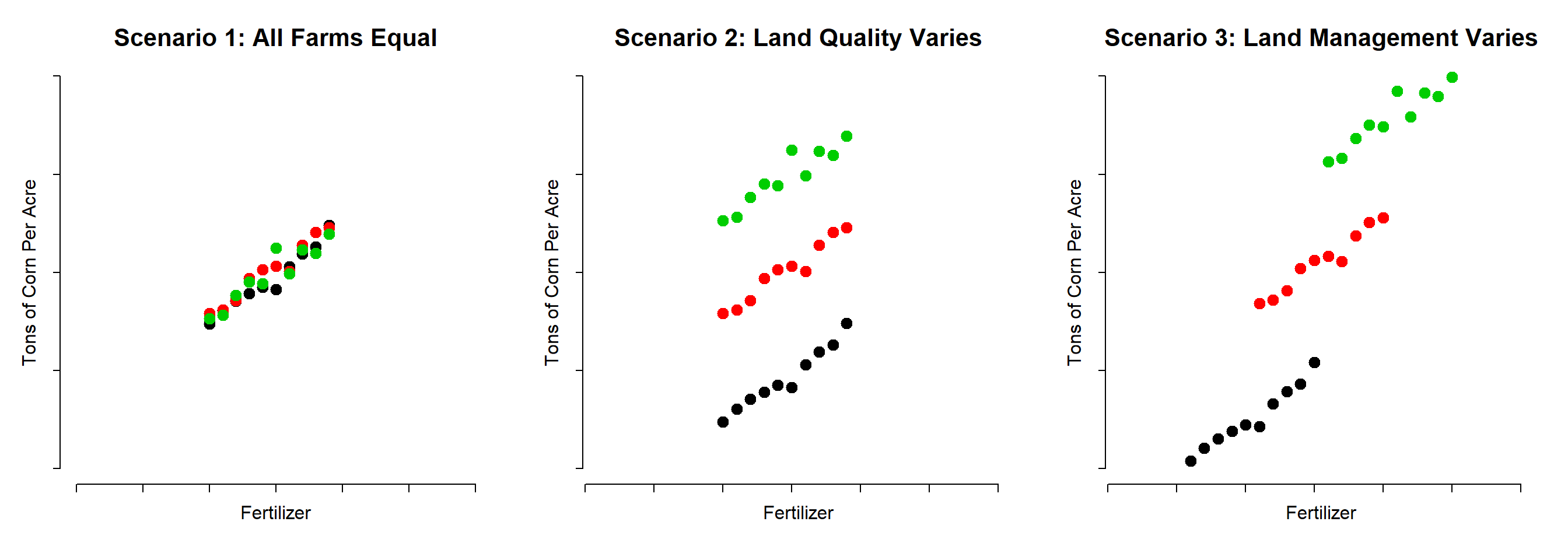
par( mfrow=c(1,3), mar=c(5.1, 4.1, 4.1, 15) )

plot( x1, y1, pch=19, col=gray(0.5,0.5), cex=3,
      ylim=c(20,70), xlim=c(0,25),
      bty="n", axes=F,
      xlab="Pooled Model is UNBIASED + EFFICIENT", ylab="",
      line=1.5, cex.lab=1.5, col.lab="gray20", cex.lab=1.5 )
axis( side = 1, labels = FALSE )
axis( side = 2, labels = FALSE )
title( main="Scenario 1", line=1, cex.main=2 )
abline( m1, lwd=2 )
b <- m1$coefficients
mtext( "  Pooled Model", side=4, outer=F, at=b[1]+25*b[2]+3, cex=1.5, las=2 )


plot( x2, y2, pch=19, col=gray(0.5,0.5), cex=3,
      ylim=c(20,70), xlim=c(1,25),
      bty="n", axes=F,
      xlab="Pooled Model is UNBIASED + INEFFICIENT", ylab="",
      line=1.5, cex.lab=1.5, col.lab="gray20", cex.lab=1.5 )
axis( side = 1, labels = FALSE )
axis( side = 2, labels = FALSE )
title( main="Scenario 2", line=1, cex.main=2 )
abline( m2.ols, lwd=2 )
for(i in 1:3){ abline( lm(y2[id==i]~x2[id==i]), lty=3, lwd=3, col="darkgray" ) }

# mtext( " OLS Slope", side=4, outer=F, at=m2.ols$fitted.values[30]+3, cex=1.5, las=2 )
b <- m2.re$coefficients
mtext( "  RE Slope", side=4, outer=F, at=b[1]+25*b[2]+2, cex=1, las=2 )
mtext( "  Pooled Model", side=4, outer=F, at=b[1]+25*b[2]+b[3]+2, cex=1.5, las=2 )
mtext( "  RE Slope", side=4, outer=F, at=b[1]+25*b[2]+b[4]+2, cex=1, las=2 )


plot( x3, y3, pch=19, col=gray(0.5,0.5), cex=3,
      ylim=c(20,70), xlim=c(1,25),
      bty="n", axes=F,
      xlab="Pooled Model is BIASED + INEFFICIENT", ylab="",
      line=1.5, cex.lab=1.5, col.lab="gray20", cex.lab=1.5 )
axis( side = 1, labels = FALSE )
axis( side = 2, labels = FALSE )
title( main="Scenario 3", line=1, cex.main=2 )
abline( m3.ols, lwd=2 )
for(i in 1:3){ abline( lm(y3[id==i]~x3[id==i]), lty=3, lwd=3, col="darkgray" ) }

mtext( " Pooled Model", side=4, outer=F, at=m3.ols$fitted.values[30]+5, cex=1.5, las=2 )
b <- m3.fe$coefficients
mtext( "  FE Slope", side=4, outer=F, at=b[1]+25*b[2]+2, cex=1, las=2 )
mtext( "  FE Slope", side=4, outer=F, at=b[1]+25*b[2]+b[3]+2, cex=1, las=2 )
mtext( "  FE Slope", side=4, outer=F, at=b[1]+25*b[2]+b[4]+2, cex=1, las=2 )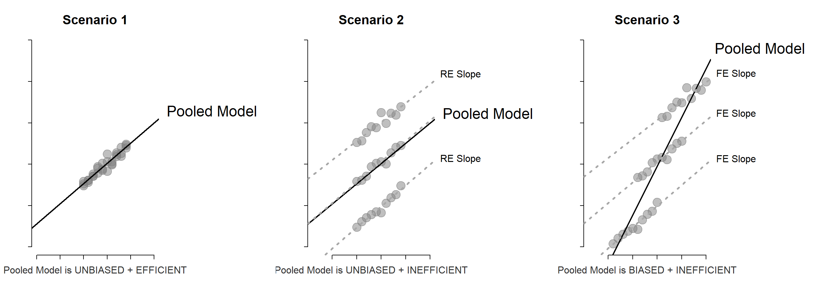
stargazer( m1, m2.ols, m2.re, m3.ols, m3.fe, m4,
           type="text",
           intercept.bottom=FALSE,
           column.labels   = c("Scenario 1", "Scenario 2", "Scenario 3"),
           column.separate = c(1,2,3),
           add.lines = list(c("True Slope",
                              "1","1","1","1","1","1"),
                            c("Fixed Effects?","NO","NO","YES","NO","YES","NO"),
                            c("Dynamic Model","NO","NO","NO","NO","NO","YES") ),
           omit=c("Constant","org.id"),
           omit.stat=c("f","ser","adj.rsq","rsq","n"),
           dep.var.labels.include = FALSE,
           dep.var.caption = "",
           digits=2 )
stargazer( m1, m2.ols, m2.re, m3.ols, m3.fe, m4,
type="html",
intercept.bottom=FALSE,
column.labels = c("Scenario 1", "Scenario 2", "Scenario 3"),
column.separate = c(1,2,3),
add.lines = list(c("True Slope",
"1","1","1","1","1","1"),
c("Fixed Effects?","NO","NO","YES","NO","YES","NO"),
c("Dynamic Model","NO","NO","NO","NO","NO","YES") ),
omit=c("Constant","org.id"),
omit.stat=c("f","ser","adj.rsq","rsq","n"),
dep.var.labels.include = FALSE,
dep.var.caption = "",
digits=2,
out="Baseline.doc")| Scenario 1 | Scenario 2 | Scenario 3 | ||||
| (1) | (2) | (3) | (4) | (5) | (6) | |
| x | 0.98*** | 0.98* | 0.98*** | 2.36*** | 0.98*** | 0.13 |
| (0.06) | (0.55) | (0.05) | (0.19) | (0.05) | (0.14) | |
| y.lagged | 0.94*** | |||||
| (0.05) | ||||||
| True Slope | 1 | 1 | 1 | 1 | 1 | 1 |
| Fixed Effects? | NO | NO | YES | NO | YES | NO |
| Dynamic Model | NO | NO | NO | NO | NO | YES |
| Note: | p<0.1; p<0.05; p<0.01 | |||||
2 TIME EFFECTS
time.effect <- rep( c(-1,1,2,3,2,1,0,-1,-2,0), 3 )
e.new <-
  c(0.717752254188994, 1.46351044875319, 0.545085270634742, 0.398709885310457,
  0.509880154168709, 1.12550062156401, -1.38757100156204, 0.199452611009322,
  0.909229008764255, -0.191497620829187, 1.92890813350955, -0.195505507481137,
  -0.206714709910741, 0.700838318157092, -0.651743403883677, 0.743503199376542,
  1.07098487453718, -0.298184876026821, -0.322110555305533, 1.33356616169561,
  2.22524178992114, 0.34393523837206, -0.00781897594284145, -0.454827433881235,
  1.91734908738423, 2.51779087685677, 0.066017323821991, 0.345542463689957,
  0.258480442909562, 0.415665805192596)
e2 <- e.new + time.effect
time <- factor( rep( 2001:2010, 3 ) )


# MODEL ZERO - NO TIME EFFECTS

x0  <- 9 + 1:10 + 0*id
y0  <- 25 + x1 + 0*id + e.new


x <- x0
y <- y0
m0.ols <- lm( y ~ x )
m0.time <- lm( y ~ x + time )


# MODEL 1 - OLS

x1  <- 9 + 1:10 + 0*id
y1  <- 25 + x1 + 0*id + e2


x <- x1
y <- y1
m1.ols <- lm( y ~ x )
m1.time <- lm( y ~ x + time )


# MODEL 2 - Random Effect

x2  <- 9 + 1:10 + 0*id
y2  <- 5 + x2 + 10*id + e2

x <- x2
y <- y2
m2.ols <- lm( y ~ x )
m2.re <- lm( y ~ x + org.id )
m2.time <- lm( y ~ x + org.id + time )


# MODEL 3

x3  <- 1:10 + 5*id
y3  <- 5 + x3 + 10*id + e2

x <- x3
y <- y3
m3.ols <- lm( y ~ x )
m3.fe <- lm( y ~ x + org.id )
m3.time <- lm( y ~ x + org.id + time )


# MODEL 4 - Dynamic

y4 <- y3[c(F,rep(T,9))]
y.lagged <- y3[c(rep(T,9),F)]
x4 <- x3[c(F,rep(T,9))]
time2 <- factor( rep( 2002:2010, 3 ) )

x <- x4
y <- y4
m4 <- lm( y ~ x + y.lagged )
m4.time <- lm( y ~ x + y.lagged + time2 )
par( mar=c(5.1, 4.1, 4.1, 15), mfcol=c(1,2) )
plot( x0[1:30], y0[1:30], pch=19, col=gray(0.5,0.5), cex=3,
ylim=c(30,60), xlim=c(5,25),
bty="n", axes=F,
xlab="Steady Growth", ylab="",
line=1.5, cex.lab=1.5, col.lab="gray20", cex.lab=1.5 )
axis( side = 1, labels = FALSE )
axis( side = 2, labels = FALSE )
title( main="Case A: No Time Effects", line=1, cex.main=2 )
abline( m0.ols, lwd=2 )
b <- m0.ols$coefficients
mtext( " OLS Model", side=4, outer=F, at=b[1]+25*b[2]-0, cex=1.5, las=2 )
abline( m0.time, col="red", lwd=2 )
mtext( " With Time Fixed Effects", side=4, outer=F, at=b[1]+25*b[2]+4, cex=1.5, las=2, col="red" )
plot( x1[1:30], y1[1:30], pch=19, col=gray(0.5,0.5), cex=3,
ylim=c(30,60), xlim=c(5,25),
bty="n", axes=F,
xlab="Boom-Bust Cycles", ylab="",
line=1.5, cex.lab=1.5, col.lab="gray20", cex.lab=1.5 )
axis( side = 1, labels = FALSE )
axis( side = 2, labels = FALSE )
title( main="Case B: Time Effects", line=1, cex.main=2 )
abline( m1.ols, lwd=2 )
b <- m1.ols$coefficients
mtext( " OLS Model", side=4, outer=F, at=b[1]+25*b[2]-0, cex=1.5, las=2 )
abline( m1.time, col="red", lwd=2 )
mtext( " With Time Fixed Effects", side=4, outer=F, at=b[1]+25*b[2]+4, cex=1.5, las=2, col="red" )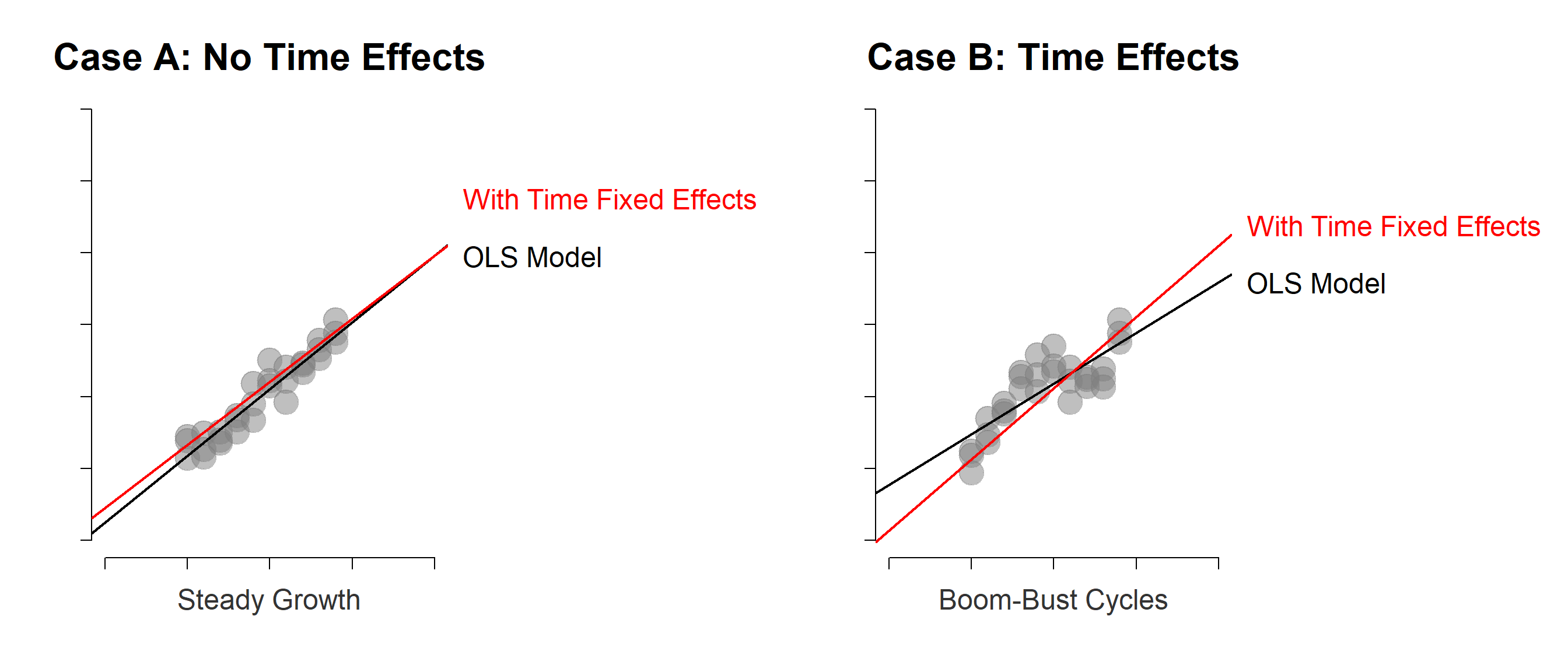
stargazer( m1.ols, m1.time, m2.re, m2.time, m3.fe, m3.time,
           type="text",
           intercept.bottom=FALSE,
           column.labels   = c("Scenario 1", "Scenario 2", "Scenario 3"),
           column.separate = c(2,2,2),
           add.lines = list(c("True Slope",
                              "1","1","1","1","1","1"),
                            c("Org Fixed Effects?",
                              "YES","YES","YES","YES","YES","YES"),
                            c("Time Fixed Effects?",
                              "NO","YES","NO","YES","NO","YES") ),
           omit=c("org.id","time","time2"),
           omit.stat=c("f","ser","adj.rsq","rsq","n"),
           dep.var.labels.include = FALSE,
           dep.var.caption = "",
           digits=2 )
stargazer( m1, m1.time, m2.re, m2.time, m3.fe, m3.time,
type="html",
intercept.bottom=FALSE,
column.labels = c("Scenario 1", "Scenario 2", "Scenario 3"),
column.separate = c(2,2,2),
add.lines = list(c("True Slope",
"1","1","1","1","1","1"),
c("Org Fixed Effects?",
"YES","YES","YES","YES","YES","YES"),
c("Time Fixed Effects?",
"NO","YES","NO","YES","NO","YES") ),
omit=c("Constant","org.id","time","time2"),
omit.stat=c("f","ser","adj.rsq","rsq","n"),
dep.var.labels.include = FALSE,
dep.var.caption = "",
digits=2,
out="TimeFixedEffects.doc")| Scenario 1 | Scenario 2 | Scenario 3 | ||||
| (1) | (2) | (3) | (4) | (5) | (6) | |
| x | 0.98*** | 0.99*** | 0.70*** | 0.99*** | 0.70*** | 0.99*** |
| (0.06) | (0.08) | (0.10) | (0.08) | (0.10) | (0.08) | |
| True Slope | 1 | 1 | 1 | 1 | 1 | 1 |
| Org Fixed Effects? | YES | YES | YES | YES | YES | YES |
| Time Fixed Effects? | NO | YES | NO | YES | NO | YES |
| Note: | p<0.1; p<0.05; p<0.01 | |||||
par( mfrow=c(1,3) )

plot( x1, y1, pch=19, col=org.id, cex=2,
      ylim=c(20,60), xlim=c(0,30),
      bty="n", axes=F,
      xlab="Fertilizer", ylab="Tons of Corn Per Acre",
      line=1.5, cex.lab=1.5 )
axis( side = 1, labels = FALSE )
axis( side = 2, labels = FALSE )
title( main="Scenario 1: All Farms Equal", line=1, cex.main=2 )

plot( x2, y2, pch=19, col=org.id, cex=2,
      ylim=c(20,60), xlim=c(1,30),
      bty="n", axes=F,
      xlab="Fertilizer", ylab="Tons of Corn Per Acre",
      line=1.5, cex.lab=1.5 )
axis( side = 1, labels = FALSE )
axis( side = 2, labels = FALSE )
title( main="Scenario 2: Land Quality Varies", line=1, cex.main=2 )

plot( x3, y3, pch=19, col=org.id, cex=2,
      ylim=c(20,60), xlim=c(1,30),
      bty="n", axes=F,
      xlab="Fertilizer", ylab="Tons of Corn Per Acre",
      line=1.5, cex.lab=1.5 )
axis( side = 1, labels = FALSE )
axis( side = 2, labels = FALSE )
title( main="Scenario 3: Management Varies", line=1, cex.main=2 )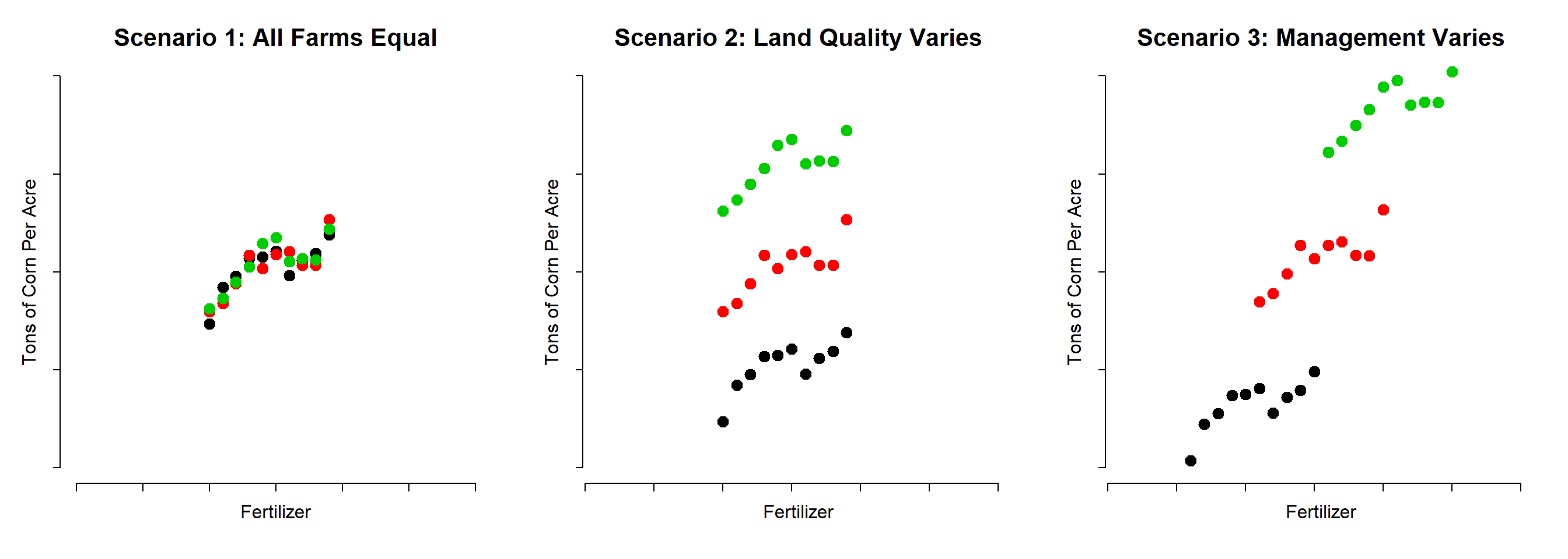
3 FIXED EFFECTS BY DE-MEANING DATA
# MODEL 1 - OLS

x1  <- 9 + 1:10 + 0*id
y1  <- 25 + x1 + 0*id + e

x <- x1
y <- y1
m1.ols <- lm( y ~ x )


# MODEL 3

x3  <- 1:10 + 5*id
y3  <- 5 + x3 + 10*id + e

x3.mean <- ave( x3, org.id )
x3.centered <- x3 - x3.mean

y3.mean <- ave( y3, org.id )
y3.centered <- y3 - y3.mean

x <- x3
y <- y3
m3.ols <- lm( y ~ x )
m3.fe <- lm( y ~ x + org.id )

x <- x3.centered
y <- y3.centered
m3.centered <- lm( y ~ x )
stargazer( m1.ols, m3.fe, m3.centered,
type="text",
intercept.bottom=FALSE,
column.labels = c("OLS on Data w No Groups",
"FE on Data w Groups",
"OLS on De-Meaned Data"),
column.separate = c(1,1,1),
add.lines = list(c("True Slope",
"1","1","1") ),
omit=c("Constant","org.id","time","time2"),
omit.stat=c("f","ser","adj.rsq","rsq","n"),
dep.var.labels.include = FALSE,
dep.var.caption = "",
digits=2 )stargazer( m1.ols, m3.fe, m3.centered,
type="html",
intercept.bottom=FALSE,
column.labels = c("OLS on Data <br> w No Groups",
"FE on Data <br> w Groups",
"OLS on <br> De-Meaned Data"),
column.separate = c(1,1,1),
add.lines = list(c("True Slope",
"1","1","1") ),
omit=c("Constant","org.id","time","time2"),
omit.stat=c("f","ser","adj.rsq","rsq","n"),
dep.var.labels.include = FALSE,
dep.var.caption = "",
digits=2,
out="DemeanedData.doc" )|
OLS on Data w No Groups |
FE on Data w Groups |
OLS on De-Meaned Data |
|
| (1) | (2) | (3) | |
| x | 0.98*** | 0.98*** | 0.98*** |
| (0.06) | (0.05) | (0.05) | |
| True Slope | 1 | 1 | 1 |
| Note: | p<0.1; p<0.05; p<0.01 | ||
## GRAPHICS

par( mfrow=c(1,3) )

plot( x1, y1, pch=19, col=gray(0.5,0.5), cex=3,
      ylim=c(34,46), xlim=c(mean(x1)-5,mean(x1)+5),
      bty="n", axes=F,
      xlab="", ylab="",
      cex.lab=1.5 )
axis( side = 1, cex.axis=2, at=c(10.5,12.5,14.5,16.5,18.5), labels=c(10,12,14,16,18) )
axis( side = 2, cex.axis=2 )
title( main="Scenario 1: No Group Structure)", line=1, cex.main=2 )
abline( h=40, lty=3, col="gray", lwd=3 )
abline( v=mean(x), lty=3, col="gray", lwd=3 )
text( 17, 39, expression( paste( "( ", bar( x ), " , ", bar( y ), " )" ) ),
      cex=2, col="black" )


plot( x3, y3,
      pch=19, col=gray(0.5,0.5), cex=3,
      ylim=c(20,60), xlim=c(1,30),
      bty="n", axes=F,
      xlab="", ylab="",
      cex.lab=1.5 )
axis( side = 1, cex.axis=2 )
axis( side = 2, cex.axis=2 )
title( main="Baseline FE Data", line=1, cex.main=2 )
for( i in 1:3 )
{
   segments( x0=min(x3[id==i])-1, x1=max(x3[id==i])+1,
             y0=mean(y3[id==i]),
             lty=3, col="gray", lwd=3 )

   segments( x0=mean(x3[id==i]),
             y0=min(y3[id==i])-1, y1=max(y3[id==i])+1,
             lty=3, col="gray", lwd=3 )

   text( mean(x3[id==i])-3, mean(y3[id==i])+3,
         expression( paste( "( ", bar( x )[j], " , ", bar( y )[j], " )" ) ),
         cex=1.5, col="black" )
}


plot( x3.centered, y3.centered,
      pch=19, col=gray(0.5,0.5), cex=3,
      ylim=c(-6,6),
      bty="n", axes=F,
      xlab="", ylab="",
      cex.lab=1.5 )
axis( side = 1, cex.axis=2 )
axis( side = 2, cex.axis=2 )
title( main="Mean Centered FE Data", line=1, cex.main=2 )
abline( h=0, lty=3, col="gray", lwd=3 )
abline( v=0, lty=3, col="gray", lwd=3 )
text( -2.3, 1.5, expression( paste( "( ", x[ij] - bar( x )[j], " , ", y[ij] - bar( y )[j], " )" ) ),
      cex=2, col="black" )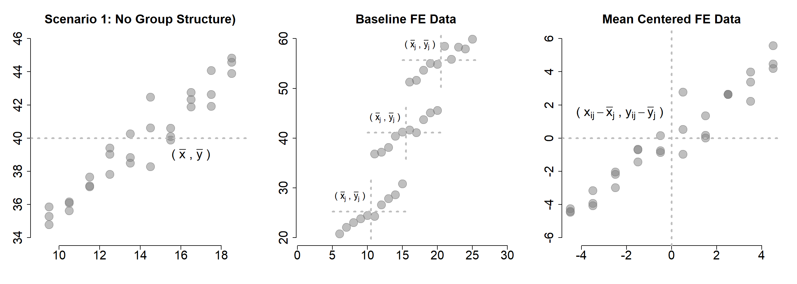
4 TAXONOMY OF BIAS FROM GROUP STRUCTURE
# SIMPSON'S PARADOX


# MODEL 1 - OLS

x1  <- 9 + 1:10 + 0*id
y1  <- 25 + x1 + 0*id + e


x <- x1
y <- y1
m1 <- lm( y ~ x )


# MODEL 2 - Random Effect

x2  <- 9 + 1:10 + 0*id
y2  <- 5 + x2 + 10*id + e


x <- x2
y <- y2
m2.ols <- lm( y ~ x )
m2.re <- lm( y ~ x + org.id )


# FE CASE 1

x11  <- 1:10 + 5*id
y11  <- 5 + x11 + 10*id + e

x <- x11
y <- y11
m11.ols <- lm( y ~ x )
m11.fe <- lm( y ~ x + org.id )


# FE CASE 2

x12  <- 1:10 + 5*id
y12  <- 10 + 15*id + e

x <- x12
y <- y12
m12.ols <- lm( y ~ x )
m12.fe  <- lm( y ~ x + org.id )


# FE CASE 3

x13  <- 1:10 + 5*id
y13  <- 60 + x13 - 18*id + e

x <- x13
y <- y13
m13.ols <- lm( y ~ x )
m13.fe  <- lm( y ~ x + org.id )


## GRAPHICS

par( mfrow=c(1,3) )


plot( x11, y11, pch=19, col=org.id, cex=2,
      ylim=c(20,60), xlim=c(0,30),
      bty="n", axes=F,
      xlab="Hours of Private Tutoring", ylab="Math Scores",
      line=1.5, cex.lab=1.5 )
axis( side = 1, labels = FALSE )
axis( side = 2, labels = FALSE )
title( main="Matthew Effect", line=1, cex.main=2 )


plot( x12, y12, pch=19, col=org.id, cex=2,
      ylim=c(20,60), xlim=c(1,30),
      bty="n", axes=F,
      xlab="Hours of Private Tutoring", ylab="Math Scores",
      line=1.5, cex.lab=1.5 )
axis( side = 1, labels = FALSE )
axis( side = 2, labels = FALSE )
title( main="Artificial Program Impact", line=1, cex.main=2 )


plot( x13, y13, pch=19, col=org.id, cex=2,
      ylim=c(20,60), xlim=c(1,30),
      bty="n", axes=F,
      xlab="Hours of Private Tutoring", ylab="Math Scores",
      line=1.5, cex.lab=1.5 )
axis( side = 1, labels = FALSE )
axis( side = 2, labels = FALSE )
title( main="Simpson's Paradox", line=1, cex.main=2 )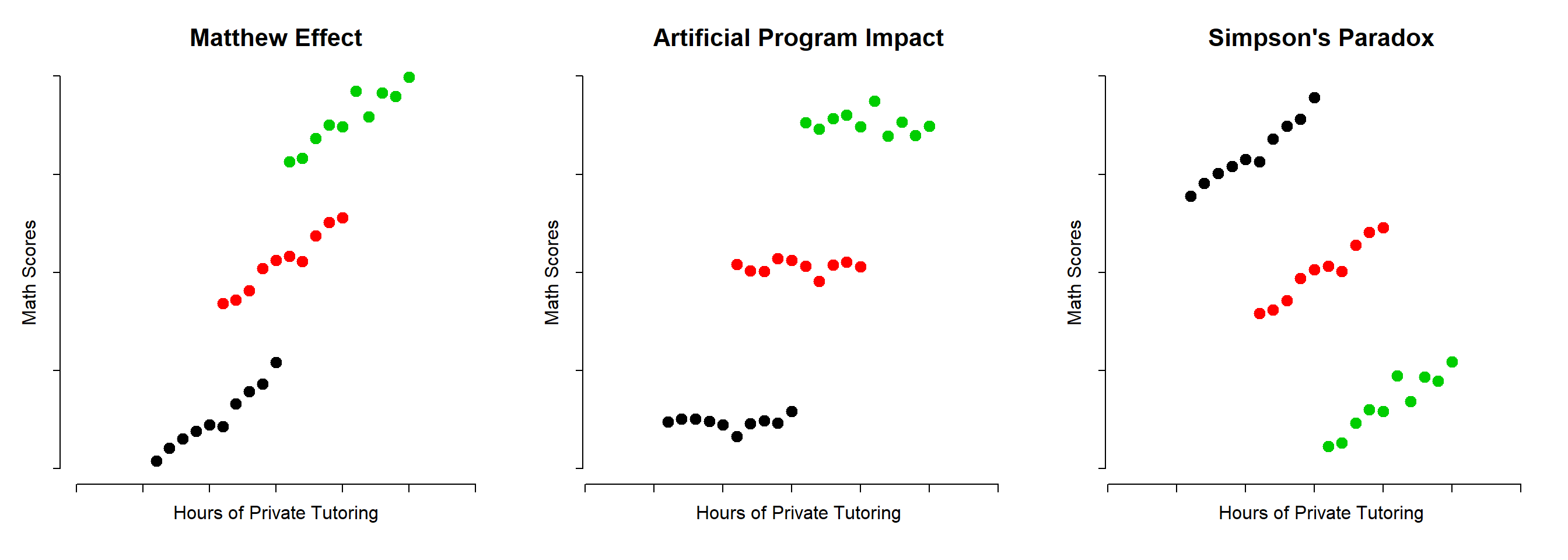
###


par( mfrow=c(1,3), mar=c(5.1, 4.1, 4.1, 15) )

plot( x11, y11, pch=19, col=gray(0.5,0.5), cex=3,
      ylim=c(20,70), xlim=c(1,25),
      bty="n", axes=F,
      xlab="Program Impact Over-Stated", ylab="",
      line=1.5, cex.lab=1.5, col.lab="gray50", cex.lab=1.5 )
axis( side = 1, labels = FALSE )
axis( side = 2, labels = FALSE )
title( main="Matthew Effect", line=1, cex.main=2 )
abline( m11.ols, lwd=2 )
for(i in 1:3){ abline( lm(y11[id==i]~x11[id==i]), lty=3, lwd=3, col="darkgray" ) }

mtext( " Pooled Model", side=4, outer=F, at=m11.ols$fitted.values[30]+5, cex=1.5, las=2 )
b <- m11.fe$coefficients
mtext( "  FE Slope", side=4, outer=F, at=b[1]+25*b[2]+2, cex=1, las=2 )
mtext( "  FE Slope", side=4, outer=F, at=b[1]+25*b[2]+b[3]+2, cex=1, las=2 )
mtext( "  FE Slope", side=4, outer=F, at=b[1]+25*b[2]+b[4]+2, cex=1, las=2 )


plot( x12, y12, pch=19, col=gray(0.5,0.5), cex=3,
      ylim=c(20,70), xlim=c(1,25),
      bty="n", axes=F,
      xlab="Program Impact Over-Stated", ylab="",
      line=1.5, cex.lab=1.5, col.lab="gray50", cex.lab=1.5 )
axis( side = 1, labels = FALSE )
axis( side = 2, labels = FALSE )
title( main="Artificial Program Impact", line=1, cex.main=2 )
abline( m12.ols, lwd=2 )
for(i in 1:3){ abline( lm(y12[id==i]~x12[id==i]), lty=3, lwd=3, col="darkgray" ) }

mtext( " Pooled Model", side=4, outer=F, at=m12.ols$fitted.values[30]+5, cex=1.5, las=2 )
b <- m12.fe$coefficients
mtext( "  FE Slope", side=4, outer=F, at=b[1]+25*b[2]+2, cex=1, las=2 )
mtext( "  FE Slope", side=4, outer=F, at=b[1]+25*b[2]+b[3]+2, cex=1, las=2 )
mtext( "  FE Slope", side=4, outer=F, at=b[1]+25*b[2]+b[4]+2, cex=1, las=2 )


plot( x13, y13, pch=19, col=gray(0.5,0.5), cex=3,
      ylim=c(20,70), xlim=c(1,25),
      bty="n", axes=F,
      xlab="Impact has Wrong Sign", ylab="",
      line=1.5, cex.lab=1.5, col.lab="gray50", cex.lab=1.5 )
axis( side = 1, labels = FALSE )
axis( side = 2, labels = FALSE )
title( main="Simpson's Paradox", line=1, cex.main=2 )
abline( m13.ols, lwd=2 )
for(i in 1:3){ abline( lm(y13[id==i]~x13[id==i]), lty=3, lwd=3, col="darkgray" ) }

mtext( " Pooled Model", side=4, outer=F, at=m13.ols$fitted.values[30]-3, cex=1.5, las=2 )
b <- m13.fe$coefficients
mtext( "  FE Slope", side=4, outer=F, at=b[1]+25*b[2]+2, cex=1, las=2 )
mtext( "  FE Slope", side=4, outer=F, at=b[1]+25*b[2]+b[3]+2, cex=1, las=2 )
mtext( "  FE Slope", side=4, outer=F, at=b[1]+25*b[2]+b[4]+2, cex=1, las=2 )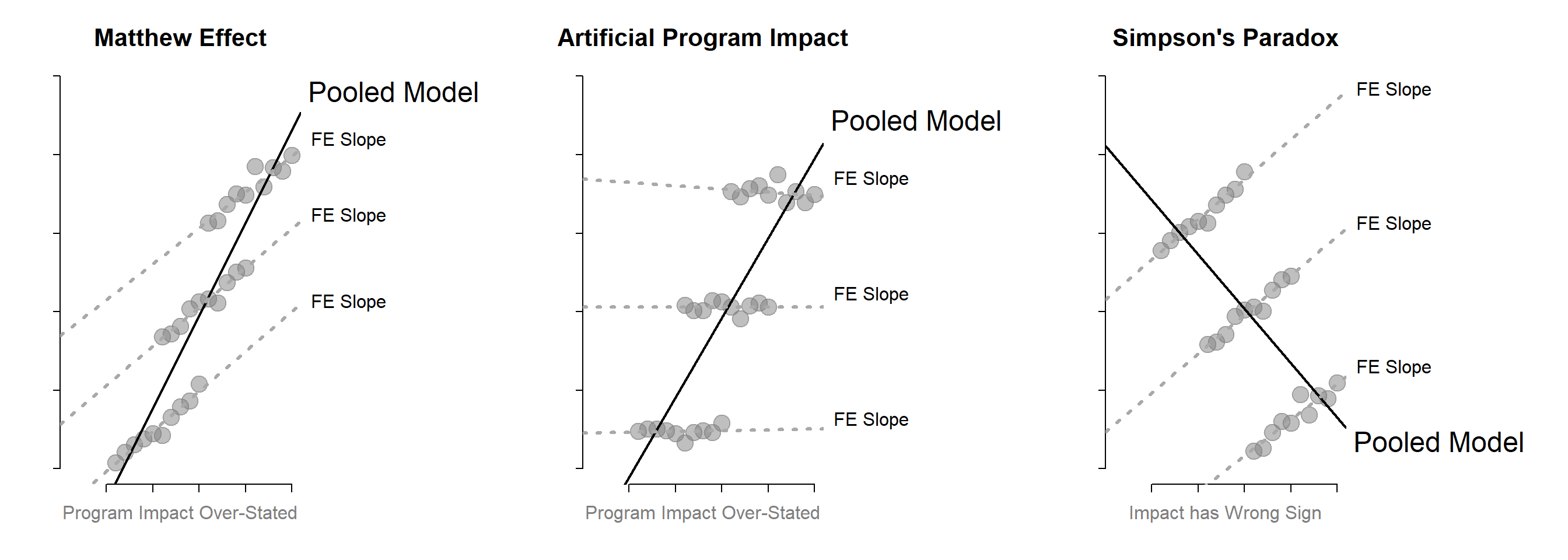
stargazer( m11.ols, m11.fe, m12.ols, m12.fe, m13.ols, m13.fe,
           type="text",
           intercept.bottom=TRUE,
           column.labels   = c("Matthew Effect",
                               "Artificial Impact",
                               "Simpson's Paradox"),
           column.separate = c(2,2,2),
           add.lines = list(c("True Slope",
                              "1","1","0","0","1","1"),
                            c("Fixed Effects?",
                              "NO","YES","NO","YES","NO","YES") ),
           omit=c("Constant","org.id","time","time2"),
           omit.stat=c("f","ser","adj.rsq","rsq","n"),
           dep.var.labels.include = FALSE,
           dep.var.caption = "",
           digits=2 )
stargazer( m11.ols, m11.fe, m12.ols, m12.fe, m13.ols, m13.fe,
type="html",
intercept.bottom=TRUE,
column.labels = c("Matthew Effect",
"Artificial Impact",
"Simpson's Paradox"),
column.separate = c(2,2,2),
add.lines = list(c("True Slope",
"1","1","0","0","1","1"),
c("Fixed Effects?",
"NO","YES","NO","YES","NO","YES") ),
omit=c("Constant","org.id","time","time2"),
omit.stat=c("f","ser","adj.rsq","rsq","n"),
dep.var.labels.include = FALSE,
dep.var.caption = "",
digits=2,
out="BiasModels.doc")| Matthew Effect | Artificial Impact | Simpson’s Paradox | ||||
| (1) | (2) | (3) | (4) | (5) | (6) | |
| x | 2.36*** | 0.98*** | 2.03*** | -0.02 | -1.39*** | 0.98*** |
| (0.19) | (0.05) | (0.27) | (0.05) | (0.32) | (0.05) | |
| True Slope | 1 | 1 | 0 | 0 | 1 | 1 |
| Fixed Effects? | NO | YES | NO | YES | NO | YES |
| Note: | p<0.1; p<0.05; p<0.01 | |||||