Chapter 5 The Regression Slope
5.1 Variance Revisited
Recall from Unit 2 we discussed the variability and variance of the data. We therefore are intersted in how the data is spread out from the mean of the data. To assess how the data is spread out from the mean we want a measure for how spread out or how the data deviates from the mean \(\bar{x}\) This is accomplished by using the following calculation: \(\Sigma(x_{i} - \bar{x})\), which is the summation of the deviation of each data point from the mean. The complete formula for calculating the variance is Eq. 5.1
Eq. 5.1 \(\sigma^2 = \Sigma(x_{i} - \bar{x})^2)/(n-1)\)
We also saw that if you add all of the deviations from the mean, the distance from the mean of each data point, it will always be \(0\). To solve this problem of the sum of the deviations being \(0\) we squared each deviation, which you can see in Eq. 5.1.
5.2 The Standard Deviation Revisited
Recall that we calculated the standard deviation by taking the square root of the variance. This is necessary because the squared deviations from the mean are in squared units. However, the original data and the mean are not in squared units. Taking the square root of the variance it puts the standard deviation in the original units.
5.2.1 Squared Residuals
Related to the variace, we minimized the sum of the squared residuals, or the distance of each data point from the regression line. This will give us the best estimation for the regression line.
5.3 Covariance
So far we have discussed how the data varies around the mean and varies around the regression line. Often we are interested in how two variables vary together. In otherwords, as one variable increase does the other variable increase or decrease. How two variables vary with each other is called the covariance. This is related to regression slopes. If the regression slope is positive then as the independent variable increases the dependent variable increases. If the regression slope is negative then as the independent variable increases the dependent variable decreases.
5.3.1 Calculating The Covariance
The equation for the covariance will look similar to that of the variance. With the variance we calculated the sum of the squared deviations from the mean. However, with covariance we have two variables. For the covariance we now calculate the sum of the deviations of the two variables multiplied together, variable \(1\) or \(x\) and variable \(2\) or \(y\), Eq. 5.2. While similar to the next step in the variance, for the covariance we now add the multiplied deviations of \(x\) and \(y\), Eq. 5.3.
Eq. 5.2
\((x_{i} - \bar{x})(y_{i} - \bar{y})\)
Eq. 5.3
\(\Sigma(x_{i} - \bar{x})(y_{i} - \bar{y})\)
Finally we divide by \(n-1\), or the sample size minus 1. Eq. 5.4. \(cov(x,y)\) stands for the covariance. Let us look at Eq. 5.4 more closely. A positive number multiplied by a positive number will result in a positive number. Therefore if \((x_{i} - \bar{x})\) and \((y_{i} - \bar{y})\) are either both positive or both negative then the numerator and thus the covariance will be positive. Alternatively, if \((x_{i} - \bar{x})\) is positive and \((y_{i} - \bar{y})\) is negative than the numerator and thus the covariance will be negative. The third possibility is if \((x_{i} - \bar{x})\) is negative and \((y_{i} - \bar{y})\) is positive than the numerator and thus the covariance will be also be negative.
Eq. 5.4
\(cov(x,y)=\Sigma(x_{i} - \bar{x})(y_{i} - \bar{y})/n-1\)
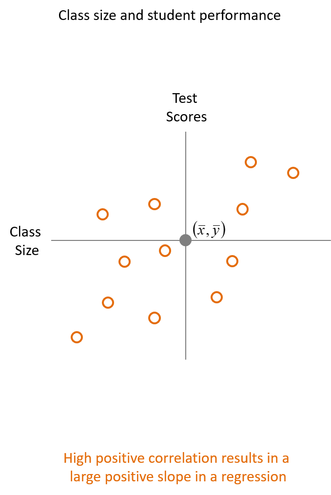
We can use the covariance to calculate the correlation between two variables. Corrlation measures the strength of the linear relationship and the direction between two variables. Suppose we were interested in how class size, the independent variable, is related to test scores, the dependent variable. If there is a positive covariance and correlation between the the two variables will increase from bottom left to upper right in a plot, Fig. 5.1.
5.3.2 Positive Correlation
Fig. 5.1
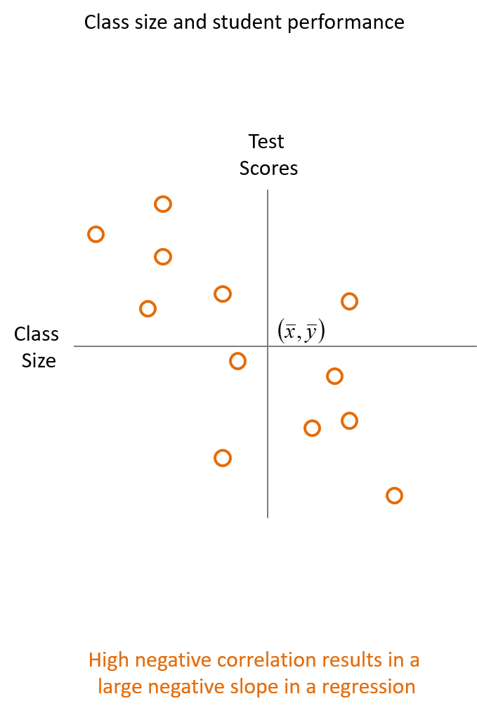
5.3.3 Negative Corrleation
If there is a negative covariance and correlation between the the two variables will decrease from top left to bottom right in a plot,
Fig. 5.2
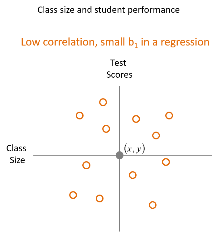
5.3.4 Low Correlation
If there is a low to no covariance and correlation (the variables are unrelated) between the the two variables will appear randomly scatterd in the plot with no upward or downward to the right, Fig. 5.3. There are two other possibilitties. If the plot is either arranged in a vertical or horizontal pattern then there is also no correlation. This is because the vertical plot means as \(y\) increases then \(x\) does not change and the horizontal plot means as \(x\)increases \(y\) does not change.
Correlations are always between \(-1\) and \(+1\). If the the correlation is closer to \(1\), then the correlation is positive and has a strong linear relationship. If the correlation is closer the correlation is to \(-1\), then the correlation is negative and has a strong linear relationship. Finally, if the correlation is closer to \(0\), then the correlation is low and has a weak linear relationship. A correlation of \(0\) would mean that the variables are completely unrelated.
5.4 The Slope
Recall the equations for the covariance and variance: Eq. 5.4 and Eq. 5.1. We can divide the covariance by the variance as seen in Eq. 5.5. With a little algebra \((n-1)\) in both the covariance and variance will cancel out each other. This will leave us with \([(\Sigma(x_{i} - \bar{x})(y_{i}) - \bar{y})]/[\Sigma(x_{i} - \bar{x})^2)]\). By cancelling each \(\Sigma(x_{i} - \bar{x})\) in the numerator and denominator we are left with the components in Eq. 5.6. This is an intuitive formula for the slope because, if you recall from algebra the slope of a line is the change in \(y\) divided by the change in \(x\).
Eq. 5.5 \(cov(x,y)/var(x)=[\Sigma(x_{i} - \bar{x})(y_{i} - \bar{y})/n-1]/[\Sigma(x_{i} - \bar{x})^2)/(n-1)]\)
Eq. 5.6 \((y_{i} - \bar{y})/(x_{i} - \bar{x})\)
5.5 Looking Ahead
We will discuss how the variance can be explained with partitioning different variaces
We will discuss \(R^2\) or the coefficient of determination