COURSE CONTENT:
- Course Overview
- Week 1 - Introduction to Project Management
- Week 2 - Data Management
- Week 3 - Analysis of Neighborhood Change
- Week 4 - Predicting Neighborhood Change
- Week 5 - Adding Federal Data
- Week 6 - Bringing it all together
- Week 7 - Finalizing Deliverables
Course Overview
Course Cadence
The project will be split into the following steps:
- Week 1: Neighborhood Revitalization Background
- Week 2: Build the Census Dataset
- Week 3: Descriptive Analysis
- Week 4: Model Neighborhood Change
- Week 5: Construct Measures of Neighborhood Health
- Week 6: Estimate Program Impact
- Week 7: Finalize Deliverables
These analysis will mirror with following project management steps:
- Week 1: Introduction to Project Management
- Week 2: Build an R Data Package
- Week 3: Document the Data
- Week 4: Draft Report
- Week 5: Format Report / Add Citations
- Week 6: Interpret Models
- Week 7: Finalize Deliverables
Week 1 - Introduction to Project Management
Due Tuesday, October 20th
Post by Friday, October 16th
Week 2 - Data Management
Building a Neighborhood Change Database
In this project we are ultimately interested in building models to explain neighborhood change between 1990 and 2010.
Census data is central to this analysis. We have begun using the harmonized Longitudinal Tracts Data Base, and by now you understand the challenges of working with the data.
This unit covers the remaining data steps necessary to wrangle the harmonized census data into a meaningful format necessary to conduct descriptive analysis.
Background Material
CRISP-DM is a useful checklists used for planning data-driven projects.
Cross-industry standard process for data mining (CRISP-DM) describes six major iterative phases, each with their own defined tasks and set of deliverables such as documentation and reports.
- Business Understanding: determine business objectives; assess situation; determine data mining goals; produce project plan
- Data Understanding: collect initial data; describe data; explore data; verify data quality
- Data Preparation (generally, the most time-consuming phase): select data; clean data; construct data; integrate data; format data
- Modeling: select modeling technique; generate test design; build model; assess model
- Evaluation: evaluate results; review process; determine next steps
- Deployment: plan deployment; plan monitoring and maintenance; produce final report; review project
Each step in the model is designed to help a team anticipate tasks in the data analytics process.
This phase of the class project focuses on the following task lists in CRISP-DM:
Data Understanding
The second stage consists of collecting and exploring the input dataset. The set goal might be unsolvable using the input data, you might need to use public datasets, or even create a specific one for the set goal.
- Collect Initial Data
- Initial Data Collection Report
- Describe Data
- Data Description Report
- Explore Data
- Data Exploration Report
- Verify Data Quality
- Data Quality Report
Data Preparation
As we all know, bad input inevitably leads to bad output. Therefore no matter what you do in modeling — if you made major mistakes while preparing the data — you will end up returning to this stage and doing it over again.
- Select Data
- The rationale for Inclusion/Exclusion
- Clean Data
- Data Cleaning Report
- Construct Data
- Derived Attributes
- Generated Records
- Integrate Data
- Merged Data
- Format Data
- Reformatted Data
- Dataset Description
Reference Material:
Note that the name uses the phrase “for data mining”, but it is a general framework for data science projects that was developed when “data mining” was a popular term used to describe an emerging field. In the metaphor the data is the rich medium that analysts mine for insights about business processes. The term has fallen out of favor because mining sounds atheoretical. Computer scientists were criticized for developing algorithms that can detect patterns and make predictions without any understanding of the processes or contexts, often leading to ethically questionable recommendations or problematic recommendations. The phrase “data science” was adopted to convey that there is a method to the madness. The CRISP-DM process applies broadly to most data science projects.
For a slightly more extensive list of tasks at each phase, see:
Examples of Integration of the CRISP-DM Process in R
CRISP-DM is one example of a project task-list, but not the only option. You will find that the R community has started incorporating some of these process models / project management tools into R packages:
Portability & Version Control
Fundamentally, portability and version control are all about making sure that other people are:
- able to re-run your code; and
- establish a clear history of edits that make it possible to identify, communicate, and ultimately resolve bugs in your code.
These concepts will be enforced through four tools:
- RStudio Projects;
- The renv package;
- The .gitignore file; and
- Version control techniques via GitHub.
Slide deck & transcript
This week will be the most demanding in terms of learning and directly applying what is covered in this week’s videos. To break up the videos into digestable pieces of content, each tool is covered in two types of videos: lectures & tutorials.
All content covered in each of these videos is documented in this Presentation. All transcripts from each lecture are preserved in the Document.
The videos are presented in the order that they should be watched:
Intro to WK02 Concepts
Intro to Portability & RStudio Projects
Lecture:
Tutorial:
renv package
Lecture:
Tutorial:
.gitignore file
Lecture:
Tutorial:
Git Feature Branch Workflow
Lecture:
Tutorial:
Lab Overview
This lab demonstrates a very minor redesign of the Longitudinal Tracts Database files to make the rest of the project smoother.
Variable names are standardized, files combined, meta-data on tracts made accessible, and a harmonization file is created to make it much faster and easier to use variables within the ten datasets.
You will follow the steps that were deployed to accomplish this, build a new data dictionary that has a more intuitive structure, and create a couple of functions to operationalize a more intuitive work flow with the data.
Data
You will find the Census Longitudinal Tabulated Database (LTDB) file here:
Harmonized Census Data Part-01
Harmonized Census Data Part-02
Most of the variables you need will come from the first dataset, which is comprised of variables that come from the long-form version of the census (which is only administered to a sample of the population) or variables from the American Community Survey (the annual survey given to a subsample of citizens).
The second dataset contains only variables that come from the Dicennial Census short form, and thus they are population measures and not sample estimates.
Set Up Your Directory Structure
While working on Lab-02 start building out your directory structure for your project. Below is an example of the folders and sub-folders you’ll need to make:
. (root/main/project directory)
├── README.md
├── analysis
│   └── README.md
├── assets
│   ├── README.md
│   ├── css
│   │   └── README.md
│   └── images
│       └── README.md
├── <RStudio Project Label>.Rproj
├── data
│   ├── README.md
│   ├── raw
│   │   ├── LTDB-DATA-DICTIONARY.xlsx
│   │   ├── LTDB-codebook.pdf
│   │   ├── LTDB_County_1980_Global_Neighborhood.csv
│   │   ├── LTDB_County_1990_Global_Neighborhood.csv
│   │   ├── LTDB_County_2000_Global_Neighborhood.csv
│   │   ├── LTDB_County_2010_Global_Neighborhood.csv
│   │   ├── LTDB_Std_1970_fullcount.csv
│   │   ├── LTDB_Std_1980_fullcount.csv
│   │   ├── LTDB_Std_1990_fullcount.csv
│   │   ├── LTDB_Std_2000_fullcount.csv
│   │   ├── LTDB_Std_2010_fullcount.csv
│   │   ├── LTDB_Std_All_Sample.zip
│   │   ├── LTDB_Std_All_fullcount.zip
│   │   ├── README.md
│   │   ├── cbsa-crosswalk.rds
│   │   ├── ltdb_data_dictionary.csv
│   │   ├── ltdb_std_1970_sample.csv
│   │   ├── ltdb_std_1980_sample.csv
│   │   ├── ltdb_std_1990_sample.csv
│   │   ├── ltdb_std_2000_sample.csv
│   │   └── ltdb_std_2010_sample.csv
│   ├── rodeo
│   │   ├── LTDB-1970.rds
│   │   ├── LTDB-1980.rds
│   │   ├── LTDB-1990.rds
│   │   ├── LTDB-2000.rds
│   │   ├── LTDB-2010.rds
│   │   ├── LTDB-META-DATA.rds
│   │   └── README.md
│   └── wrangling
│       └── README.md
├── labs
│   ├── wk01
│       └── README.md
│   ├── wk02
│       └── README.md
│   ├── wk03
│       └── README.md
│   ├── wk04
│       └── README.md
│   ├── wk05
│       └── README.md
│   ├── wk06
│       └── README.md
│   └── wk07
│       └── README.md
Consider each lab as a chapter in the book that is your final group website
You need to provide careful documentation of how you get from raw data in your project to final results. Think about it as a book where each chapter covers a distinct task:
- Identifying indicators of gentrification
- Descriptive analysis of neighborhood change
- Community demographics that predict revitalization
- Impact of federal programs
- Packaging of final deliverables
You will activate the GitHub page option for your repository and use the main landing page as the executive summary and index for HTML files that you generate in R Studio from your analysis.
For example, this was a project students did with the Syracuse Land Bank to help them identify data that could be used to target rehabilitation projects:
https://lecy.github.io/SyracuseLandBank/
And another guide describing how you might document the journey from raw data to the final dataset that you use for your analysis. Every step should be explicit, and you should openly discuss the how and why of data wrangling:
https://github.com/jtleek/datasharing
Each folder should contain it’s own README.md file with notes on what the folder contains.
Documenting Your Data Steps
Start creating a guide to use of the data in this project.
Raw Files
All of the raw data files will go in the raw folder. By “raw” we mean the data as it arrived from whatever site we retrieved it from, or the file exactly how it was exported from a custom data collection tool like an online survey program.
Anything that documents the data collection process lives here. This folder also contain scripts used to download data from APIs or scripts that scrape data from websites. Also include any documentation of source data files like data dictionaries or guides to use.
If you are using data from third-party sources make sure you document retrieval dates, URLs, and to the extent possible any parameters that were used when downloading the data. Scripts are preferable because the arguments are then documented and the behavior can be replicated. If you have to manually enter a bunch of parameters in a data download GUI on the website then if there are questions about the raw data it is never possible to fully replicate the process. It will be unclear whether the provide updated the database and the data files changed, or whether the user incorrectly entered some parameters.
Common errors at the download step include things like making an error on a Census variable name (easy to do since the raw names are things like *B19013*). Or alternatively, incorrectly applying a filter like geography or time-period during a download.
Depending on how many unique data sources you use, you may want to include subdirectories for each unique source.
Data Wrangling
This folder documents the process of converting raw data into the “rodeo” dataset you use for your models and descriptive statistics. Data steps include:
- Data cleaning
- Recoding
- Variable transformations
- Data aggregation
- Merging files
- Filters
- Conversion from long to wide formats or vice-versa
Data aggregation typically means changing the unit of analysis. If you have a database of all crimes in a city for a given year but the rest of your data is at the census tract level, you can aggregate up from individual crimes to a count by census tract so that you can add the measure to your dataset.
There are many ways that you can introduce errors while preparing your data, but be extra careful when merging (“joining”) or filtering datasets. These are steps where you can easily drop lots of observations without realizing it and introduce bias into your models through a hidden selection process.
For example, when applying filters always check to make sure data has been standardized. For example, are all city names written the same? “New York” vs “New York City” vs “NYC” could cause problems. What happens in a filter if a name is typed with an extra space: “NYC “?
Always inspect levels of categorical variables before merges or filters:
sort( unique( x ) )    # variable stored as a character vector
sort( levels( x ) )    # variable stored as a factor
The final step of the data wrangling scripts should be to save the new data file into the rodeo folder.
You might generate several files that are used at the modeling stage. As a rule of thumb, if the file is used to create descriptive statistics or for any models in your analysis it should be saved in the rodeo folder.
Rodeo Data
This folder contains datasets that have been cleaned and processed, and are ready for analysis. Typically in your RMD scripts used to produce all of the results in your reports you will read data primarily from the rodeo folder.
This allows us to isolate errors made in preparing the data (data wrangling) from errors made during the modeling stages.
You should not be doing data wrangling in your analytical steps with the exception of variable transformations related to modeling. For example, creating a squared value of a variable X to use in a quadratic model, logging a variable, or dividind by a constant to change the unit of analysis. Since these are steps related directly to the modeling process it is helpful to keep them together.
Due on Tuesday, October 27th
YellowDig Topic
Refining a Theory of Neighborhood Change
The first step in the CRISP-DM model is developing a “Business Understanding” of the problem. In evaluation we will refer to this step as defining our theory of change for the program - how we believe the program or project is creating impact.
This stage is aimed toward getting a general understanding of the client’s business. It is crucial in most cases to understand the application of the product to be developed. If it is skipped — you might end up with a great solution for a problem that does not exist.
- Determine Business Objectives
- Background
- Business Objectives
- Business Success Criteria
- Assess the Situation
- Inventory of Resources
- Requirements, Assumptions, and Constraints
- Risks and Contingencies
- Terminology
- Costs and Benefits
- Determine Goals
- Data Mining Goals
- Data Mining Success Criteria
- Produce Project Plan
- Project Plan
- Initial Assessment of Tools and Techniques
In evaluation I would add steps that emphasize the importance of identifying the primary outcomes or dependendent variables of the study.
Goals of Development Assistance
The federal programs under consideration are one of many programs that consist of “aid” or “assistance” dollars being sent to vulnerable communities to catalyze some sort of change.
One of my favorite data viz fails is this tone-def visualization of World Bank contracts presented by adapting what appears to be a World War III missile attack simulation. Development aid is launched from the donor country and explodes as it hits the recipient country:
The metaphor is perfect for todays discussion topic because the science of economic development is still in the leaches phase and many argue that some policies do more harm than good.
It is important to identify clear goals or outcomes for these programs in order to build a theory of change around the intended impact and start to operationalize measures for outcomes.
The Great Debate - People vs Places
There is a long-standing debate in urban policy. Should we spend money helping people? Or should we spend money helping the places where disadvantaged people live? Neighborhood revitalization strategies target the latter.
Ed Glaeser, a renouned urban economist, makes the argument for people provacatively in the articles, Should the government rebuild New Orleans or just write residents checks and Can Buffalo ever come back
(his answers are write a check, and instead of subsidizing Buffalo residents to live in an unproductive geography we should use the money to help them move to Atlanta)
He is exagerating a bit to highlight the peverse incentives inherent in a lot of economic development funding. He is a little more even-handed in the academic article titled, “The Economics of Place-Making Policies”:
“Should the national government undertake policies aimed at strengthening the economies of particular localities or regions? …any government spatial policy is as likely to reduce as to increase welfare …most large-scale place-oriented policies have had little discernable impact. Some targeted policies such as Empowerment Zones seem to have an effect but are expensive relative to their achievements. The greatest promise for a national place-based policy lies in impeding the tendency of highly productive areas to restrict their own growth through restrictions on land use.”
There are detractors that would argue Glaeser is wrong, many programs do work (for example see Revitalizing Inner-City Neighborhoods: New York City’s Ten-Year Plan and Building Successful Neighborhoods ). I suspect Glaeser’s response would be that exceptional success cases do not prove that the typical intervention produces intended (or large average) effects, and that even when they do work they are expensive relative to other alternatives.
In their essay, Who Benefits From Neighborhood Improvements?. Strong Towns makes an even stronger argument while cautioning about the unintended consequences of policy instruments created to promote development. After they exist they can be coopted by developers in order to capture some of the most valuable land in the city by taking it from poor residents:
The “shell [neighborhoods]” referred to above do not simply ‘appear’ as part of some naturally-occurring neighbourhood ‘decay’ – they are actively produced by clearing out existing residents via all manner of tactics and legal instruments, such as landlord harassment, massive rent increases, redlining, arson, the withdrawal of public services, and eminent domain/compulsory purchase orders. Closing the rent gap requires, crucially, separating people currently obtaining use values from the present land use providing those use values – in order to capitalise the land to the perceived ‘highest and best’ use.
So while Glaeser argues that place-based policies like neighborhood revitalization can be inefficient, Strong Towns argues that even worse they can be used against the residents that they were created to help.
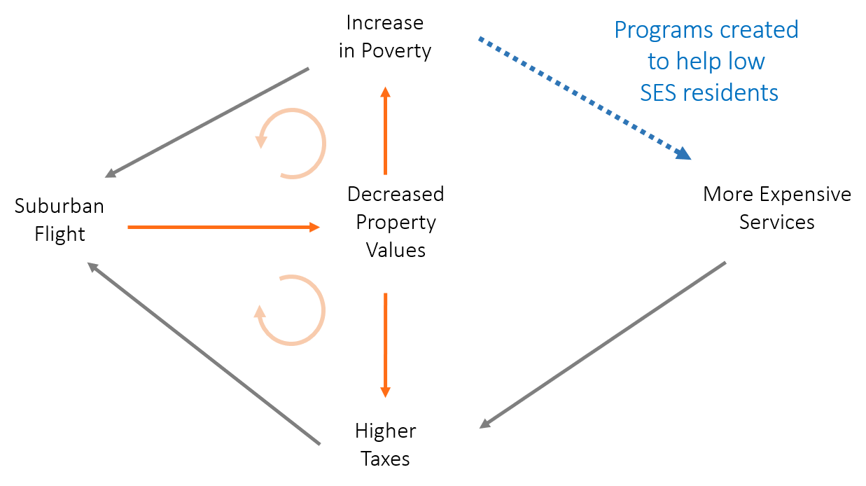
This is not the only example of intended effects of community improvement policies. In the book Making Cities Work Robert Inman highlights the trade-off between policies that strengthen the middle class in neighborhoods to keep them from becoming poor and keeping the community strong versus those that target the poor. Anti-poverty measures can enhance a white flight feedback loop that consequently can lead to higher concentrations of poverty in cities.
From the study by Haughwout and his colleagues (2004), summarized in table 11.3, we learn that in the four sample cities, higher taxes depress city property values and reduce jobs within the city, even allowing for the possibly positive effect of increased revenues on city services. The analysis is specified so that the effect of taxes on the tax base includes any offsetting effects added revenues might have from allowing more spending on valued city services.
The estimated negative effect of taxes on property values suggests there is a “fiscal gap” between the costs of the taxes paid and the benefits received by those buying property in the city. It is significant. Haughwout and his colleagues (2004) estimate that Houston and New York City property owners receive no additional benefits from the last dollar of property taxes paid. Philadelphia and Minneapolis property owners receive, respectively, an estimated $.43 and $.77 in added benefits from their last dollar of city taxes.’ If this last dollar is not providing sufficient benefits to taxpayers to justify its cost, where does the new tax money go?
Rather than to taxpayer services, it appears the incremental tax dollar goes to support required increases in poverty spending, public employee wages above improved worker productivity, and politically useful yet economically inefficient public projects.
The burden of city poverty on city taxpayers is twofold. First, a large poverty population implies a potentially large tax burden on middle-income households and firms. Table 11.4 shows the direct fiscal cost of cities’ own poverty spending on median household incomes for a sample of large U.S. cities. Poverty spending per capita is significant, and the implied increase in the middle-class taxes needed to fund such expenditures can be as large as 2 to 3 percent of a city’s median family income. This added tax burden is likely to drive middle-class families and firms from the city. Second, city poverty implies a possible increase in the costs of providing public services to city residents. K-12 education (Dunscombe and Yinger 1997) and resident safety (Glaeser and Sacerdote 1999) are the services whose costs are most likely to be increased by large poverty populations. Either city spending must rise or service quality must decline. Again, resident taxpayers and city firms will be tempted to leave the city. Their exit will undermine the city’s consumption and production agglomeration advantages.
As the city’s private sector economic performance declines, city and perhaps suburban property values fall. Outside grants to pay the costs of federal and state service mandates for lower-income families as well as aid for the added costs of service provision because of large concentrations of lower-income families are the appropriate policy responses. Removing the responsibility for city poverty from the city’s budget is an important first step toward greater city fiscal efficiency.
In this example the important thing to note is aid tied to families is bound by neighborhoods within cities. In effect, a poor household can only receive services if they move into central cities, whereas the same services are not offered in suburbs or wealthier neighborhoods. So it is a critique of economic apartheid more so than pro-poor policies. And even though services are provided to families they are still place-based policies and not people-based policies because they require the family to relocate to a poor neighborhood to access the services (e.g. public housing). A true people-based program would provide a voucher for the services in whichever community the household desired to live so they could follow opportunities instead of crowding into segregated and stressed census tracts (see new findings from Moving to Opportunity project).
Lack of Data
These above issues are raised not to argue that place-based initiatives are not effective or pro-poor policies are not helpful. Rather, it is to highlight the challenges of place-based economic development policy:
- We measure success of programs by the value locked in a neighborhood - mainly houses, household income, and schools.
- Census data does not tell us whether rises in value are a result of infill development which diversifies a neighborhood economically and benefits current residents, or by displacing poor people and replacing them with wealthier residents.
The challenge is that we do not have the appropriate data to really study this question. In the paper, “Designing Policies to Spur Economic Growth: How Regional Scientists Can Contribute to Future Policy Development and Evaluation” the authors make the argument that to improve policy-making we need to improve data because we currently cannot effectively measure the “treatment” in economic development - all of the investments and subsidies that occur within a tract (think of the missile launch visualization with aid coming from federal sources, state sources, and metro sources and flowing to specific census tracts), and using home value and income as outcome variables in these studies make it hard to tell which mechanism - growth or displacement - is driving the result.
In a couple of weeks you will begin to look at data on the effectiveness of tax credit programs on catalyzing economic development. These programs were selected partly because they are some of the only large-scale federal programs that have made their data available and easy to access.
The lack of data on this topic is a huge gap in the open data landscape. Only recently have serious attempts been made to measure the extent of these credits, and mostly by people outside of government, the most notable example being the Panel Database on Incentives and Taxes. But without good data on all government and private investments flowing into census tracts we are likely to produce biased evaluations of policy effectiveness.
Prediction vs Causality
If you are not feeling well the doctor might take a blood sample to test for cancer. They are looking for elevated levels of white blood counts and various protein markers. If present the doctor can detect cancer early and have a better chance of treating it effectively.
Blood markers predict cancer. They do not cause it. Doctors almost never actually know the cause of a specific case of cancer, but they know from drug trials which medicines work for treating it.
Similarly, it is much easier to predict which census tracts are likely to improve over time than it is to explain the underlying causes. In policy we care about causality because we want to know if we implement a specific expensive revitalization policy it will create the intended changes. But prediction is also useful for planning and responsible governance of the process of change.
As we move past descriptive analysis and into inferential models try to keep the two ideas distinct in your mind. Some of the census variables will help us predict which neighborhoods are likely to change over the next decade. But many of these are like blood markers - they provide information that can be used for prediction but don’t necessarily explain the mechanisms.
Our interest in tax credits, however, is causal. Saying that a model offers an unbiased estimate of program impact is the same thing as saying we have cleanly identified a causal mechanism. If you filter out white blood cells from a persons body you do not remove the cancer because the mechanism is not causal. If you increase dollars spent on revitalization in a neighborhood will you actually see more development occur?
Take caution when interpretting variables that might be markers so that you do not make the mistake of saying things like immigrants drive down home prices and school performance. The actual mechanism is more likely immigrants are located in declining neighborhoods because it’s where the cheapest housing is, but without immigrants the neighborhood would decline even faster. Correlation is not causation. Check your assumptions.
More importantly, try to think about the requirements necessary to make the claim that economic development programs cause neighborhood change. There is a big selection problem here - tax credit programs are implemented by bankers and developers. This is prudent design because they have a vested interest in the tax credits working since investments in communities where they don’t will create a loss for them. It limits wasteful spending on neighborhoods where the programs have no chance of success. On the other hand the program dollars are more likely to flow to neighborhoods that are most likely to experience growth since those are communities where return on investment is highest. As a result many resources are spent in communities where development would have occurred without the program. In this case the programs are not creating community change, and since they are likely flowing to communities that are expected to improve anyhow they are only effective if they create more change than we would have experienced without them. The counterfactual is really important in this context!
If a community is on the up-swing it will attract tax credit dollars, but it will also attract a lot of other types of investment. We can only cleanly identify the impact of tax credits if we can control for all other types of investment. Therein lies the rub.
Reflection
If you could get data on any capital expenditure or economic transfer that landed in a census tract, what data would you want to include in the model? Are there place-based investments like infrastructure or schools that you think would matter? Programs that target the type of residents that live in the community? Private investments like new businesses (Starbucks and Whole Foods) or improvements to current housing stock. Parks? Bike paths? Recreation facilities?
Assuming data is no issue, what sorts of investments would you want to include as controls in your model?
Post your reflection to YellowDig by Friday, October 23rd
Week 3 - Analysis of Neighborhood Change
For this part of the project you will:
- Using the 2000 to 2010 template, calculate change in the MHV variable between 1990 and 2000.
- Pick a city and create a new dorling cartogram to visualize your data.
- Prepare descriptive statistics and chloropleth maps describing the MHV change variable.
Background Material
Modeling
We are entering the fourth phase of the CRISP-DM Checklist by starting analysis of the data.
- Select Modeling Techniques
- Modeling Technique
- Modeling Assumptions
- Generate Test Design
- Test Design
- Build Model
- Parameter Settings
- Models
- Model Descriptions
- Assess Model
- Model Assessment
- Revised Parameter Settings
This phase emphasizes the important work of:
- Creating new variables through variable transformations
- Exploratory and descriptive analysis
- Building basic models
- Preliminary hypothesis-testing
Lab Overview
Descriptive Analysis
TUTORIAL ON DESCRIPTIVE ANALYSIS
Due on Friday, November 6th
YellowDig Topic
Revisiting Gentrification
The problem with neighborhood revitalization initiatives is it is hard to measure success using readily available census data. We want the neighborhoods to get “better”. But what does better look like? And for who?
This project emphasizes gentrification for two reasons.
One is philosophical and related to the concept of a theory of change. Neighborhood revitalization projects were designed to address the concentrated poverty and blight that has a negative impact on the community that lives there. Conceptually we would like to improve the well-being of peole in the community through the neighborhood, not simply give the neighborhood a face lift. The challenge is that if we are not careful about designing programs or measuring outcomes we will end up “improving” the neighborhood by pushing all of the residents out. For example, if we focus on things like income and educational outcomes for children, the easiest way to improve these metrics is to replace poor households that are moving with wealthier and better-educated families. This strategy is anti-thetical to the goal of improving quality of life and social mobility for residents.
The second reason why gentrification is important for this project is because it must be measured with data. You will find that if you change the defition of gentrification slightly, you can change the outcome greatly. Forcing you to operationalize gentrification in the study forces you to think critically about the data, and to pay attention to how others are using the same data.
Some recent studies have sounded the alarm that gentrification is accelerating: 20 percent of low-income communities experienced gentrification between 2000 and 2010, almost twice the rate of gentrification in the 1990s. (side note - please keep this statistic in mind for next week’s topic on urban renewal)
A recent study turns a lot of the debate on its head by using better data to track movement into and out of neighborhoods by poor families. They find that displacement caused by gentrification is way less than expected, and they call into question the way in which gentrification is measured.
Please read this short blog on the topic.
The research raises two important questions: (1) how do we measure gentrification? And (2) how prevelant is it?
In next week’s lab on descriptive analysis of census tracts you will be asked to report on the level of gentrification you observe, which requires you to measure it. Note the diversity and nuance of some approached to measurement. For example, THIS METHODOLOGY by The Urban Displacement Project uses a taxonomy of five stages of gentrification to be more precise about the process.
For your YellowDig discussion this week propose a method for operationalizing the identification of gentrification in census data using variables in the harmonized census LTDB files. Specify:
(1) The criteria used to classify a census tract as eligible to be gentrified (a tract that is already wealthy and white cannot be further gentrified).
(2) The criteria you will use to determine whether the tract experienced gentrification between 2000 and 2010.
Explain your methodology to your classmates.
Next week, after you have finished your lab report back on what level of gentrification you found. Was it more or less than you expected?
Post your reflection to YellowDig by Friday, October 30th
Week 4 - Predicting Neighborhood Change
This week you will accomplish two things: practice variable transformations and build your baseline model of neighborhood change before adding the policy variables in the next lab.
Background Reading
Introduction to models where the outcome is home value: hedonic pricing models.
The main insight is that home price is a variable that aggregates a tremendous amount of information about characteristics of houses, neighborhoods, and cities. We can use regression to separate out these difference attributes at different levels, and see they each contributes to the market value of a home.
Since we are using the median home value variable which represents an entire census tract we focus on how neighborhood attributes and changes in attributes over time impact the average home price in the tract.
Hedonic Pricing Models Overview
Hedonic Pricing Regression Example in R
Valuation Using Hedonic Pricing Models
Lab Overview
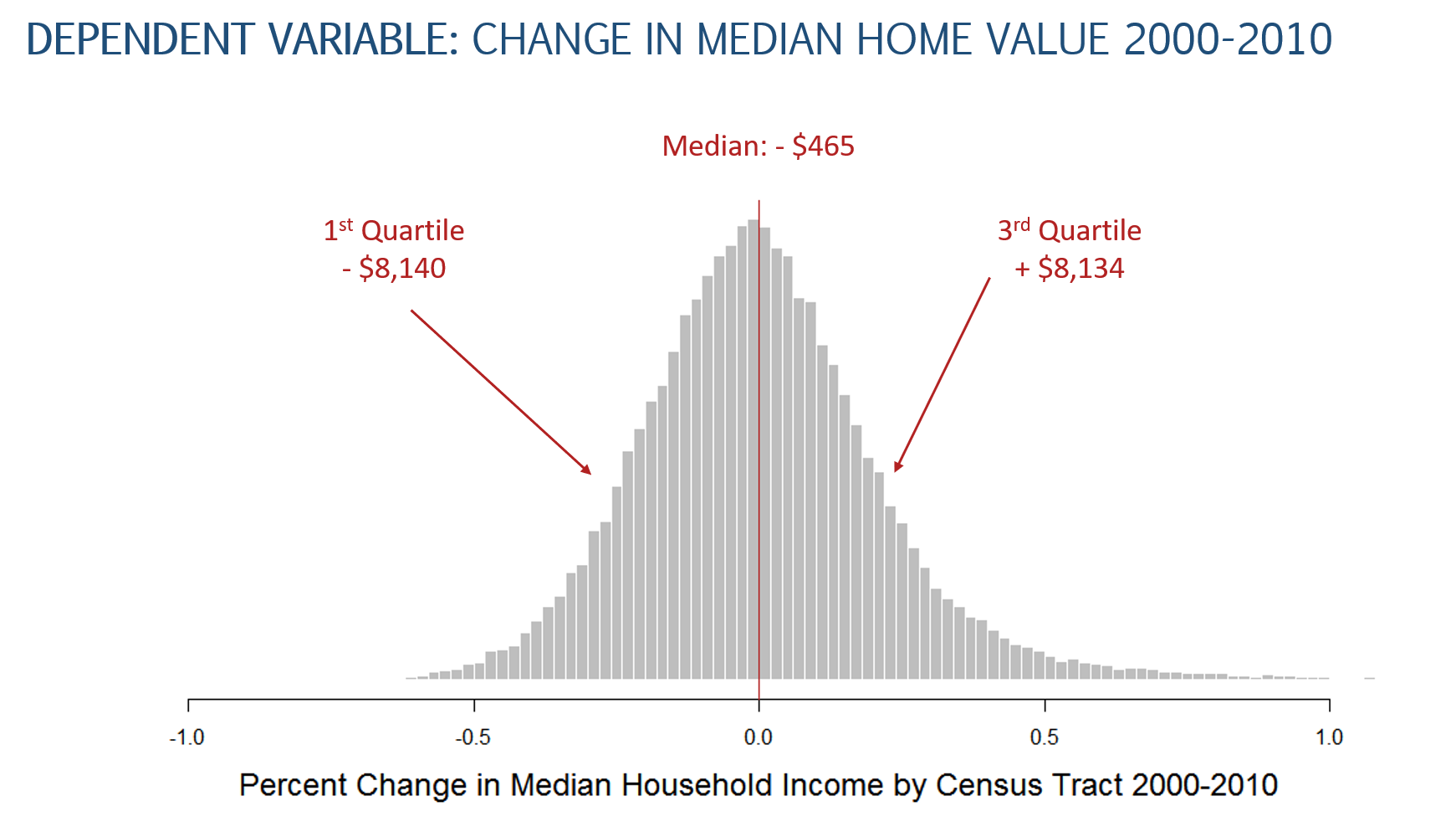
The dependent variable in our model is the median home value. The choice draws on a large body of work on “hedonic pricing models” which assert that home values are a good price mechanism to capture the state of a neighborhood because they “price in” all of the characteristics of the house as well as the features of the neighborhood and surrounding city.
TUTORIAL ON PREDICTING MHV CHANGE
Give context into why you are working on this lab and be sure to describe your methodology using R Markdown documents, showing your code for all of the steps.
Write up your results and submit your RMD file and the knitted HML version when both upload to Canvas and share with your teammates via GitHub.
Due on Tuesday, November 10th
YellowDig Discussion
Share your final models and insights on the outcome.
Which control variables did you find to best predict the revitalization in your model?
Post your reflection to YellowDig by Friday, November 6th
Week 5 - Adding Federal Data
This week offers an opportunity to analyze real-world policy data to make sense of two large federal programs.
The first part, Lab 04, asks you to build a model of home value change using census data that describes tracts in 2000 and 2010.
Lab 05 then extends this baseline model by adding data on the New Market Tax Credits (NMTC) and Low Income Housing Tax Credit (LIHTC) programs.
The labs are designed to give you experience working with real-world data and all of its flaws, and to reinforce some of the content from CPP 523, 524, and 525.
The analysis is complex, so we are looking for modest models with a small number of variables, which gives you a chance to clean up the data if necessary and spend time interpreting results.
Summary of Tax Credit Programs
Background Info on NMTC & LIHTC
Lab Overview
This last step in your project will walk you through adding data from two federal programs designed to help low-income communities.
You will use the following tutorial to add federal program data to your models. Ultimately, you will go onto use the difference-in-difference framework introduced here to estimate the impact of each program.
Lab Instructions
- Use your baseline model predicting tract change from Lab 04 as the starting point.
- Create a log-linear diff-in-diff model following these steps and add your control variables from Lab 04.
Give context into why you are working on this lab and be sure to describe your methodology using R Markdown documents, showing your code for all of the steps.
Write up your results and submit your RMD file and the knitted HML version when both upload to Canvas and share with your teammates via GitHub.
Due on Tuesday, November 17th
YellowDig Discussion
Share your final models and insights on the outcome.
Do Low Income Tax Credits seem to have an impact on home values?
Do New Market Tax Credits impact home values?
Post your reflection to YellowDig by Friday, November 13th
Week 6 - Bringing it all together
Place building blocks into the analysis/ directory
This week offers you an opportunity to finally use the analysis/ directory. As a team, you will determine which teammates’ lab will be used as the building blocks for your group website.
The reason why you’re picking one person’s lab is so that you can all agree which labs to move from the labs/ directory into the analysis/ directory. Once those labs are there, please drop the last names from the file as these are now team-owned labs.
Review the chapter requirements within the project rubric
Once selected, you should return to your project rubric and make sure you are able to add more context to write the following four documents:
- Chapter on descriptive analysis of neighborhood change
- Chapter predicting change with neighborhood characteristics
- Chapter describing tax credit programs (NMTC & LIHTC)
- Predictive models after adding tax credit programs
Deliverables
This week your team deliverable is to:
- Create a boiler plate GitHub Pages website
- Create an executive summary
- Schedule office hours with me as a team to review your work / address any point points
Due on Tuesday, November 24th
Post your reflection YellowDig:
I only have one question for you: what pain point did you experience this week? If you could go back in time, how would you resolve these problems?
Week 7 - Finalizing Deliverables
Your final week will be spent finalizing all of your project files, models, documentation, and report using GitHub sites.
There is no final presentation, so the YellowDig posts give you a chance to share your work and reflect on key components of the course.
The weekly YellowDig point restrictions have been lifted this week, so all of your activities contribute toward your final YellowDig score. Point requirements will be adjusted to account for the week without a topic.
Final Deliverables
Make sure to review the project rubric to ensure you have included all of the necessary components:
Submit to Canvas:
Collaboration Tools
Which aspects of the collaboration tools have you found useful?
Which parts have been awkward or challenging?
Do you believe the project was easier or harder using the tools?
If you were managing a large project with many waves of data, your recommendations have real consequences for how resources will be allocated through a federal program, you are the lead for a team of 7 analysts, and analysis that is complex enough that no one team member has all of the skills needed to generate the deliverables.
Does the usefulness of the project management tools change with the complexity of the project?
Post your reflection YellowDig:
How Confident Are You in Your Recommendations?
Consider all of the steps that are necessary to conduct analysis of a policy or program and make conclusions about effectiveness or recommendations on implementation:
- Developing domain expertise
- Identifying and collecting data
- Wrangling data (cleaning, aggregating, reshaping, merging)
- Operationalizing your research questions and developing appropriate measures of your key latent constructs
- Exploring and describing your data
- Selecting a model that leverages a feasible identification strategy appropriate for your data and question
- Interpretting results in a way that policy-makers can understand them
- Conducting sensitivity analysis to ensure you are confident with your recommendations
In your YellowDig post reflect on the following:
Where do you feel like you are most likely to introduce bias into the process?
Do you feel like the benefits of peer review (all work is reviewed by team members) outweigh the costs?
What was the hardest part of reviewing someone else’s code?
Post your reflection YellowDig:
Final Deliverables
Share a link to your project website and highlight specific sections when you answer the following:
What is one aspect of the project you are proud of and that you think works well?
What is one aspect of the final product that you hope to improve upon next time?
Each team member should answer individually.
Post your reflection YellowDig: