17 Data Joins

17.1 Packages Used in This Chapter

library( pander )
library( dplyr )
library( maps )

17.2 Relational Databases

Modern databases are huge - think about the amount of information stored at Amazon in the history of each transation, the database where Google logs every single search from every person around the world, or Twitter’s database of all of the tweets (millions each day).

When databases become large, flat spreadsheet style formats are not useful because they create a lot of redundant information, are large to store, and are not efficient to search. Large datasets are instead stored in relational databases - sets of tables that contain unique IDs that allow them to be joined when necessary.

For example, consider a simple customer database. We don’t want to store customer info with our transactions because we would be repeating their name and street address every time they make a new purchase. As a result, we store customer information and transaction information separately.

Customer Database

CUSTOMER.ID	FIRST.NAME	LAST.NAME	ADDRESS	ZIP.CODE
178	Alvaro	Jaurez	123 Park Ave	57701
934	Janette	Johnson	456 Candy Ln	57701
269	Latisha	Shane	1600 Penn Ave	20500

Transactions Database

CUSTOMER.ID	PRODUCT	PRICE
178	video	5.38
178	shovel	12
269	book	3.99
269	purse	8
934	mirror	7.64

If we want to make the information actionable then we need to combine these datasets. For example, perhaps we want to know the average purchase amount from an individual in the 57701 zip code. We cannot answer that question with either dataset since the zip code is in one dataset, and the price is in another. We need to merge the data.

merge( customer.info, purchases )

  CUSTOMER.ID FIRST.NAME LAST.NAME       ADDRESS ZIP.CODE PRODUCT PRICE
1         178     Alvaro    Jaurez  123 Park Ave    57701   video  5.38
2         178     Alvaro    Jaurez  123 Park Ave    57701  shovel 12.00
3         269    Latisha     Shane 1600 Penn Ave    20500    book  3.99
4         269    Latisha     Shane 1600 Penn Ave    20500   purse  8.00
5         934    Janette   Johnson  456 Candy Ln    57701  mirror  7.64

full.dat <- merge( customer.info, purchases ) 

full.dat$PRICE[ full.dat$ZIP.CODE == "57701" ]

[1]  5.38 12.00  7.64

mean( full.dat$PRICE[ full.dat$ZIP.CODE == "57701" ] )

[1] 8.34

In reality, each purchase would have a purchase ID that is linked to shipping addresses, customer complaints, seller ratings, etc. Each seller would have their own data table with info. Each purchase would be tied to a payment type, which has its own data table. The system gets quite complex, which is why it is important to pay attention to the details of putting the data back together again.

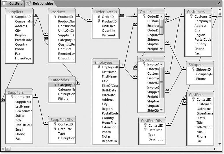
We will cover a few details of data merges that will help you avoid common and very subtle mistakes that can lead to incorrect inferences.

17.3 Set Theory

In order to merge data correctly you need to understand some very basic principles of set theory.

17.3.1 Set Theory Functions

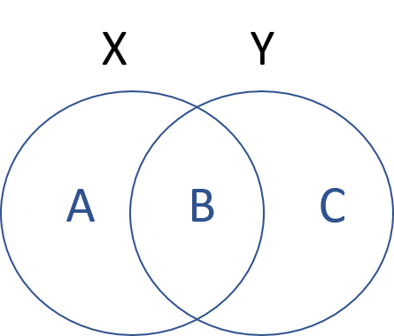
Let’s assume we have two sets: set1=[A,B], set2=[B,C]. Each element in this set represents a group of observations that occurs in the dataset. So B represents people that occur in both datasets, A represents people that occur only in the first dataset, and C represents people that only occur in the second dataset.

We can then describe membership through three operations:

Operation	Description
union: X OR Y	The universe of all elements across all both sets: [A,B,C]
intersection: X & Y	The elements shared by both sets: [B]
difference: X & ! Y	The elements in my first set, not in my second [A] or [C]

Let’s see how this might work in practice with an example of members of a study:

name	group	gender
frank	treat	male
wanda	treat	female
sanjay	control	male
nancy	control	female

For this example let’s define set 1 as the treatment group, and set 2 as all women in the study. Note that set membership is always defined as binary (you are in the set or out), but it can include multiple criteria (the set of animals can contains cats, dogs, and mice).

treated <- name[ group == "treat" ]

treated

[1] "frank" "wanda"

females <- name[ gender == "female" ]

females

[1] "wanda" "nancy"

Now we can specify group belonging using some convenient set theory functions: union(), setdiff(), and intersect().

union( treated, females )

[1] "frank" "wanda" "nancy"

intersect( treated, females )

[1] "wanda"

setdiff( treated, females )

[1] "frank"

setdiff( females, treated )

[1] "nancy"

It is very important to note that union() and intersect() are symmetric functions, meaning intersect(x,y) will give you the same result as intersect(y,x). The setdiff() function is not symmetric, however.

17.3.2 Set Theory Using Logical Operators

Typically you will define your groups using logical operators, which perform the exact same funciton as set theory functions but are a little more expressive and flexible.

Let’s use the same example above where x=“treatment” and y=“female”, then consider these cases:

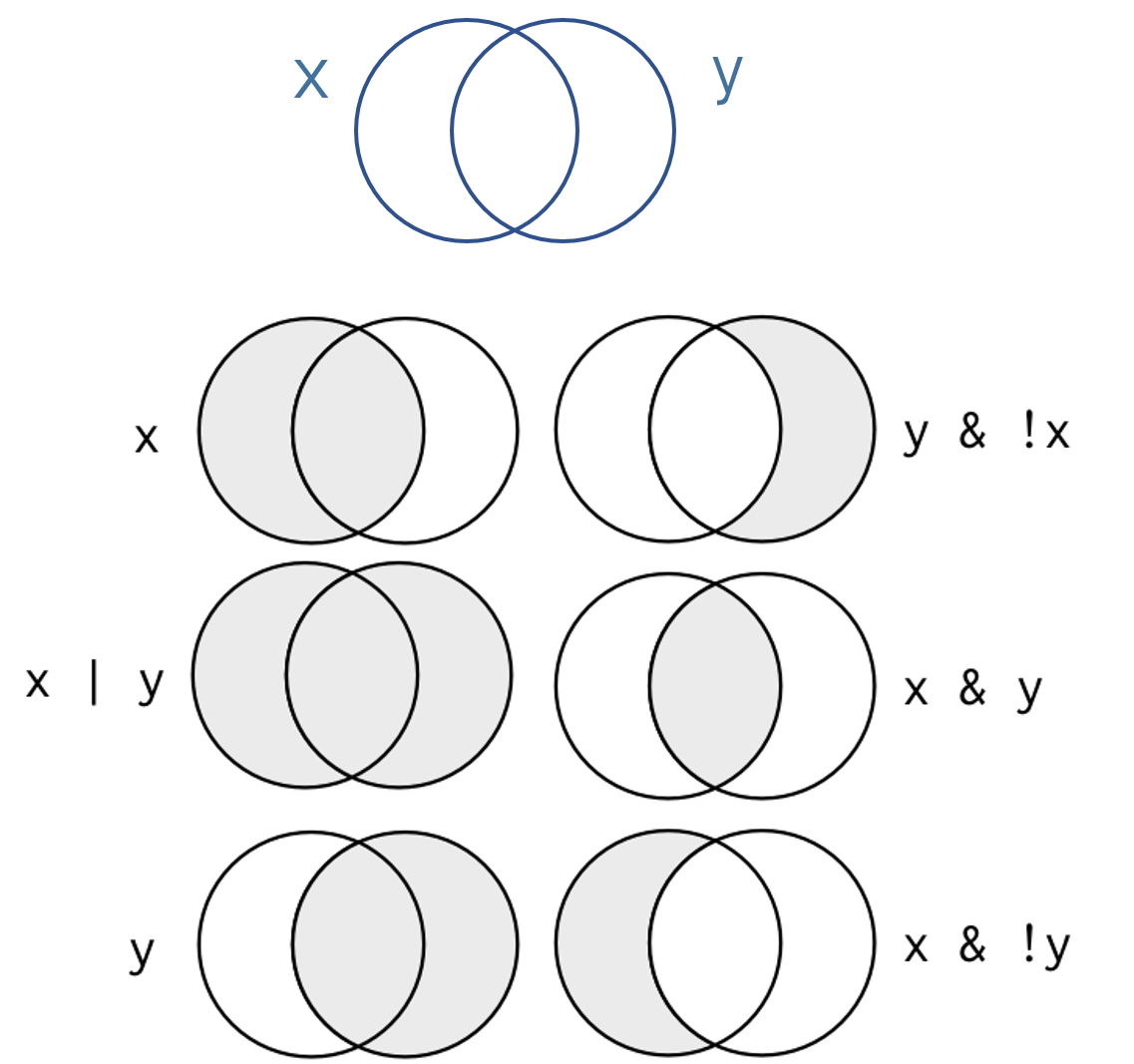
Who belongs in each group?

name	group	gender
frank	treat	male
wanda	treat	female
sanjay	control	male
nancy	control	female

#   x

name[ group == "treat" ]

[1] "frank" "wanda"

#   x & y

name[ group == "treat" & gender == "female" ]

[1] "wanda"

#   x & ! y

name[ group == "treat" & gender != "female" ]

[1] "frank"

#  x | y

name[ group == "treat" | gender == "female" ]

[1] "frank" "wanda" "nancy"

Who belongs in these groups?

!x & !y
x & ! ( x & y )
( x | y ) & ! ( x & y )

17.4 Merging Data

The Merge Function

The merge function joins two datasets. The function requires two datasets as the arguments, and they need to share a unique ID variable. Recall the example from above:

merge( customer.info, purchases )

  CUSTOMER.ID FIRST.NAME LAST.NAME       ADDRESS ZIP.CODE PRODUCT PRICE
1         178     Alvaro    Jaurez  123 Park Ave    57701   video  5.38
2         178     Alvaro    Jaurez  123 Park Ave    57701  shovel 12.00
3         269    Latisha     Shane 1600 Penn Ave    20500    book  3.99
4         269    Latisha     Shane 1600 Penn Ave    20500   purse  8.00
5         934    Janette   Johnson  456 Candy Ln    57701  mirror  7.64

The important thing to keep in mind is that the default merge operation uses the intersection of the two datasets. It will drop all elements that don’t occur in both datasets. We may want to fine-tune this as to not lose valuable data and potentially bias our analysis. As an example, no illegal immigrants will have social security numbers, so if you are merging using the SSN, you will drop this group from the data, which could impact your results.

With a little help from the set theory examples above, we can think about which portions of the data we wish to drop and which portions we wish to keep.

Argument	Usage
all=F	DEFAULT - new dataset contains intersection of X and Y (B only)
all=T	New dataset contains union of X and Y (A, B & C)
all.x=T	New dataset contains A and B, not C
all.y=T	New dataset contains B and C, not A

Here is some demonstrations with examples adapted from the R help file.

authors

      surname nationality deceased
1       Tukey          US      yes
2     Tierney          US       no
3      Ripley          UK       no
4      McNeil   Australia       no
5 Shakespeare     England      yes

books

         name                     title
1       Tukey Exploratory Data Analysis
2    Venables Modern Applied Statistics
3      Ripley        Spatial Statistics
4      Ripley     Stochastic Simulation
5      McNeil Interactive Data Analysis
6 R Core Team      An Introduction to R

# adding books to the author bios dataset  ( set B only )

merge(authors, books, by.x = "surname", by.y = "name")

  surname nationality deceased                     title
1  McNeil   Australia       no Interactive Data Analysis
2  Ripley          UK       no        Spatial Statistics
3  Ripley          UK       no     Stochastic Simulation
4   Tukey          US      yes Exploratory Data Analysis

# adding author bios to the books dataset  ( set B only )

merge(books, authors, by.x = "name", by.y = "surname")

    name                     title nationality deceased
1 McNeil Interactive Data Analysis   Australia       no
2 Ripley        Spatial Statistics          UK       no
3 Ripley     Stochastic Simulation          UK       no
4  Tukey Exploratory Data Analysis          US      yes

# keep books without author bios, lose authors without books  ( sets A and B )

merge( books, authors, by.x = "name", by.y = "surname", all.x=T )

         name                     title nationality deceased
1      McNeil Interactive Data Analysis   Australia       no
2 R Core Team      An Introduction to R        <NA>     <NA>
3      Ripley        Spatial Statistics          UK       no
4      Ripley     Stochastic Simulation          UK       no
5       Tukey Exploratory Data Analysis          US      yes
6    Venables Modern Applied Statistics        <NA>     <NA>

# keep authors without book listed, lose books without author bios   ( sets B and C )

merge( books, authors, by.x = "name", by.y = "surname", all.y=T )

         name                     title nationality deceased
1      McNeil Interactive Data Analysis   Australia       no
2      Ripley        Spatial Statistics          UK       no
3      Ripley     Stochastic Simulation          UK       no
4 Shakespeare                      <NA>     England      yes
5     Tierney                      <NA>          US       no
6       Tukey Exploratory Data Analysis          US      yes

# dont' throw out any data   ( sets A and B and C )

merge( books, authors, by.x = "name", by.y = "surname", all=T )

         name                     title nationality deceased
1      McNeil Interactive Data Analysis   Australia       no
2 R Core Team      An Introduction to R        <NA>     <NA>
3      Ripley        Spatial Statistics          UK       no
4      Ripley     Stochastic Simulation          UK       no
5 Shakespeare                      <NA>     England      yes
6     Tierney                      <NA>          US       no
7       Tukey Exploratory Data Analysis          US      yes
8    Venables Modern Applied Statistics        <NA>     <NA>

Also note that the order of your datasets in the argument list will impact the inclusion or exclusion of elements.

merge( x, y, all=F ) EQUALS merge( y, x, all=F )

merge( x, y, all.x=T ) DOES NOT EQUAL merge( y, x, all.x=T )

17.4.1 The by.x and by.y Arguments

When you use the default merge() function without specifying the variables to merge upon, the function will check for common variable names across the two datasets. If there are multiple, it will join the shared variables to create a new unique key. This might be problematic if that was not the intent.

Take the example of combining fielding and salary data in the Lahman package. If we are not explicit about the merge variable, we may get odd results. Note that they two datasets share four ID variables.

library( Lahman )
data( Fielding )
data( Salaries )

intersect( names(Fielding), names(Salaries) )

[1] "playerID" "yearID"   "teamID"   "lgID"

# merge id

int <- intersect( names(Fielding), names(Salaries) )

paste( int[1],int[2],int[3],int[4], sep="." )

[1] "playerID.yearID.teamID.lgID"

To avoid problems, be explicit using the by.x and by.x arguments to control which variable is used for the merge.

head( merge( Salaries, Fielding ) )

  yearID teamID lgID  playerID salary stint POS  G GS InnOuts  PO  A E DP PB WP
1   1985    ATL   NL barkele01 870000     1   P 20 18     221   2  9 1  0 NA NA
2   1985    ATL   NL bedrost01 550000     1   P 37 37     620  13 23 4  3 NA NA
3   1985    ATL   NL benedbr01 545000     1   C 70 67    1698 314 35 4  1  1 NA
4   1985    ATL   NL  campri01 633333     1   P 66  2     383   7 13 4  3 NA NA
5   1985    ATL   NL ceronri01 625000     1   C 91 76    2097 384 48 6  4  6 NA
6   1985    ATL   NL chambch01 800000     1  1B 39 27     814 299 25 1 31 NA NA
  SB CS ZR
1 NA NA NA
2 NA NA NA
3 65 24 NA
4 NA NA NA
5 69 29 NA
6 NA NA NA

head( merge( Salaries, Fielding, by.x="playerID", by.y="playerID" ) )

   playerID yearID.x teamID.x lgID.x  salary yearID.y stint teamID.y lgID.y POS
1 aardsda01     2010      SEA     AL 2750000     2009     1      SEA     AL   P
2 aardsda01     2010      SEA     AL 2750000     2007     1      CHA     AL   P
3 aardsda01     2010      SEA     AL 2750000     2015     1      ATL     NL   P
4 aardsda01     2010      SEA     AL 2750000     2008     1      BOS     AL   P
5 aardsda01     2010      SEA     AL 2750000     2012     1      NYA     AL   P
6 aardsda01     2010      SEA     AL 2750000     2004     1      SFN     NL   P
   G GS InnOuts PO A E DP PB WP SB CS ZR
1 73  0     214  2 5 0  1 NA NA NA NA NA
2 25  0      97  2 4 1  0 NA NA NA NA NA
3 33  0      92  0 1 1  0 NA NA NA NA NA
4 47  0     146  3 6 0  0 NA NA NA NA NA
5  1  0       3  0 0 0  0 NA NA NA NA NA
6 11  0      32  0 0 0  0 NA NA NA NA NA

17.5 Non-Unique Observations in ID Variables

In some rare instances, you will need to merge to datasets that have non-singular elements in the unique key ID variables, meaning each observation / individual appears more than one time in the data. Note that in this case, for each occurance of an observation / individual in your X dataset, you will merge once with each occurance of the same observation / individual in the Y dataset. The result will be a multiplicative expansion of the size of your dataset.

For example, if John appears on four separate rows of X, and three seperate rows of Y, the new dataset will contain 12 rows of John (4 x 3 = 12).

dataset X contains four separate instances of an individual [ X1, X2, X3, X4 ]

dataset Y contains three separate instances of an individual [ Y1, Y2, Y3 ]

After the merge we have one row for each pair:

X1-Y1
X1-Y2
X1-Y3
X2-Y1
X2-Y2
X2-Y3
X3-Y1
X3-Y2
X3-Y3
X4-Y1
X4-Y2
X4-Y3

For example, perhaps a sales company has a database that keeps track of biographical data, and sales performance. Perhaps we want to see if there is peak age for sales performance. We need to merge these datasets.

bio <- data.frame( name=c("John","John","John"),
                   year=c(2000,2001,2002),
                   age=c(43,44,45) )

performance <- data.frame( name=c("John","John","John"),
                           year=c(2000,2001,2002),
                           sales=c("15k","20k","17k") )

# correct merge

merge( bio, performance, by.x=c("name","year"), by.y=c("name","year") )

  name year age sales
1 John 2000  43   15k
2 John 2001  44   20k
3 John 2002  45   17k

# incorrect merge

merge( bio, performance, by.x=c("name"), by.y=c("name") )

  name year.x age year.y sales
1 John   2000  43   2000   15k
2 John   2000  43   2001   20k
3 John   2000  43   2002   17k
4 John   2001  44   2000   15k
5 John   2001  44   2001   20k
6 John   2001  44   2002   17k
7 John   2002  45   2000   15k
8 John   2002  45   2001   20k
9 John   2002  45   2002   17k

It is good practice to check the size (number of rows) of your dataset before and after a merge. If it has expanded, chances are you either used the wrong unique IDs, or your dataset contains duplicates.

17.5.1 Example of Incorrect Merge

Here is a tangible example using the Lahman baseball dataset. Perhaps we want to examine the relationship between fielding position and salary. The Fielding dataset contains fielding position information, and the Salaries dataset contains salary information. We can merge these two datasets using the playerID field.

If we are not thoughtful about this, however, we will end up causing problems. Let’s look at an example using Kirby Pucket.

kirby.fielding <- Fielding[ Fielding$playerID == "puckeki01" , ]

head( kirby.fielding )

       playerID yearID stint teamID lgID POS   G  GS InnOuts  PO  A E DP PB WP
83868 puckeki01   1984     1    MIN   AL  OF 128 128    3377 438 16 3  4 NA NA
85177 puckeki01   1985     1    MIN   AL  OF 161 160    4213 465 19 8  5 NA NA
86509 puckeki01   1986     1    MIN   AL  OF 160 157    4155 429  8 6  3 NA NA
87916 puckeki01   1987     1    MIN   AL  OF 147 147    3820 341  8 5  2 NA NA
89284 puckeki01   1988     1    MIN   AL  OF 158 157    4049 450 12 3  4 NA NA
90705 puckeki01   1989     1    MIN   AL  OF 157 154    3985 438 13 4  3 NA NA
      SB CS ZR
83868 NA NA NA
85177 NA NA NA
86509 NA NA NA
87916 NA NA NA
89284 NA NA NA
90705 NA NA NA

nrow( kirby.fielding )

[1] 21

kirby.salary <- Salaries[ Salaries$playerID == "puckeki01" , ]

head( kirby.salary )

     yearID teamID lgID  playerID  salary
280    1985    MIN   AL puckeki01  130000
917    1986    MIN   AL puckeki01  255000
1610   1987    MIN   AL puckeki01  465000
2244   1988    MIN   AL puckeki01 1090000
2922   1989    MIN   AL puckeki01 2000000
3717   1990    MIN   AL puckeki01 2816667

nrow( kirby.salary )

[1] 13

kirby.field.salary <- merge( kirby.fielding, kirby.salary, by.x="playerID", by.y="playerID" )

head( select( kirby.field.salary, yearID.x, yearID.y,   POS,    G,  GS, salary ) )

  yearID.x yearID.y POS   G  GS  salary
1     1984     1985  OF 128 128  130000
2     1984     1986  OF 128 128  255000
3     1984     1987  OF 128 128  465000
4     1984     1988  OF 128 128 1090000
5     1984     1989  OF 128 128 2000000
6     1984     1990  OF 128 128 2816667

nrow( kirby.field.salary )

[1] 273

21*13

[1] 273

What we have done here is taken each year of fielding data, and matched it to every year of salary data. We can see that we have 21 fielding observations and 13 years of salary data, so our resulting dataset is 273 observation pairs.

This merge also makes it difficult to answer the question of the relationship between fielding position and salary if players change positions over time.

The correct merge in this case would be a merge on a playerID-yearID pair. We can create a unique key by combining playerID and yearID using paste():

head( paste( kirby.fielding$playerID, kirby.fielding$yearID, sep=".") )

[1] "puckeki01.1984" "puckeki01.1985" "puckeki01.1986" "puckeki01.1987"
[5] "puckeki01.1988" "puckeki01.1989"

But there is a simple solution as the merge function also allows for multiple variables to be used for a merge() command.

kirby.field.salary <- merge( kirby.fielding, kirby.salary, 
                            by.x=c("playerID","yearID"), 
                            by.y=c("playerID","yearID")   )

nrow( kirby.field.salary )

[1] 20

17.6 The %in% function

Since we are talking about intersections and matches, I want to briefly introduce the %in% function. It is a combination of the two.

The intersect() function returns a list of unique matches between two vectors.

data(Salaries)
data(Fielding)
intersect( names(Salaries), names(Fielding) )

[1] "yearID"   "teamID"   "lgID"     "playerID"

The match() function returns the position of matched elements.

x <- c("A","B","C","B")

y <- c("B","D","A","F")

match( x, y )

[1]  3  1 NA  1

The %in% function returns a logical vector, where TRUE signifies that the element in y also occurs in x. In other words, does a specific element in y belong to the intersection of x,y.

This is very useful for creating subsets of data that belong to both sets.

x <- c("A","B","C")

y <- c("B","D","A","B","F","B")

y %in% x # does each element of y occur anywhere in x?

[1]  TRUE FALSE  TRUE  TRUE FALSE  TRUE

y[ y %in% x] # keep only data that occurs in both

[1] "B" "A" "B" "B"

17.7 The Match Function

Often times we do not need to merge data, we may just need sort data in one dataset so that it matches the order of another dataset. This is accomplished using the match() function.

Note that we can rearrange the order of a dataset by referencing the desired position.

x <- c("Second","Third","First")

x

[1] "Second" "Third"  "First"

x[ c(3,1,2) ]

[1] "First"  "Second" "Third"

The match() function returns the positions of matches of its first vector to the second vector listed in the arguments. Or in other words, the order that vector 2 would need to follow to match vector 1.

x <- c("A","B","C")

y <- c("B","D","A")

cbind( x, y )

     x   y  
[1,] "A" "B"
[2,] "B" "D"
[3,] "C" "A"

match( x, y )

[1]  3  1 NA

match( y, x) # not a symmetric operation!

[1]  2 NA  1

# In the y vector:
#
#  [3]=A
#  [1]=B
# [NA]=D (no match)

order.y <- match( x, y )

y[ order.y ]

[1] "A" "B" NA

We can see that match() returns the correct order to put y in so that it matches the order of x. In the re-ordered vector, the first element is the original third element A, the second element is the original first element B, and there is no third element because D did not match anything in x.

Note the order of arguments in the function:

match( data I want to match to , data I need to re-order )

We can use this position information to re-order y as follows:

x <- sample( LETTERS[1:15], size=10 )

y <- sample( LETTERS[1:15], size=10 )

cbind( x, y )

      x   y  
 [1,] "M" "H"
 [2,] "L" "K"
 [3,] "G" "N"
 [4,] "C" "J"
 [5,] "F" "D"
 [6,] "I" "A"
 [7,] "A" "L"
 [8,] "O" "O"
 [9,] "H" "M"
[10,] "J" "E"

order.y <- match( x, y )

y.new <- y[ order.y ]

cbind( x, y.new )

      x   y.new
 [1,] "M" "M"  
 [2,] "L" "L"  
 [3,] "G" NA   
 [4,] "C" NA   
 [5,] "F" NA   
 [6,] "I" NA   
 [7,] "A" "A"  
 [8,] "O" "O"  
 [9,] "H" "H"  
[10,] "J" "J"

# Note the result if you confuse the order or arguments

order.y <- match( y, x )

y.new <- y[ order.y ]

cbind( x, y.new )

      x   y.new
 [1,] "M" "M"  
 [2,] "L" NA   
 [3,] "G" NA   
 [4,] "C" "E"  
 [5,] "F" NA   
 [6,] "I" "L"  
 [7,] "A" "K"  
 [8,] "O" "O"  
 [9,] "H" "H"  
[10,] "J" NA

This comes in handy when we are matching information between two tables. For example, in GIS the map regions follow a specific order but your data does not. Create a color scheme for levels of your data, and then re-order the colors so they match the correct region on the map. In this example, we will look at unemployment levels by county.

library( maps )
data( county.fips )
data( unemp )

map( database="county" )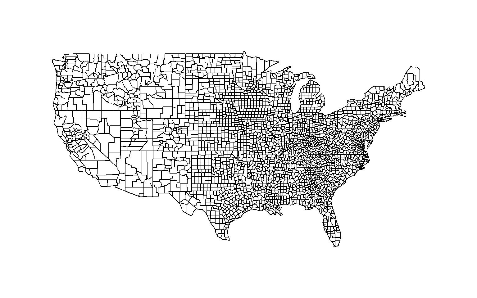

# assign a color to each level of unemployment, red = high, gray = medium, blue = low

color.function <- colorRampPalette( c("steelblue", "gray70", "firebrick") )


color.vector <- cut( rank(unemp$unemp), breaks=7, labels=color.function( 7 ) )

color.vector <- as.character( color.vector )

head( color.vector )

[1] "#B28282" "#B28282" "#B22222" "#B25252" "#B28282" "#B22222"

# doesn't look quite right

map( database="county", col=color.vector, fill=T, lty=0 )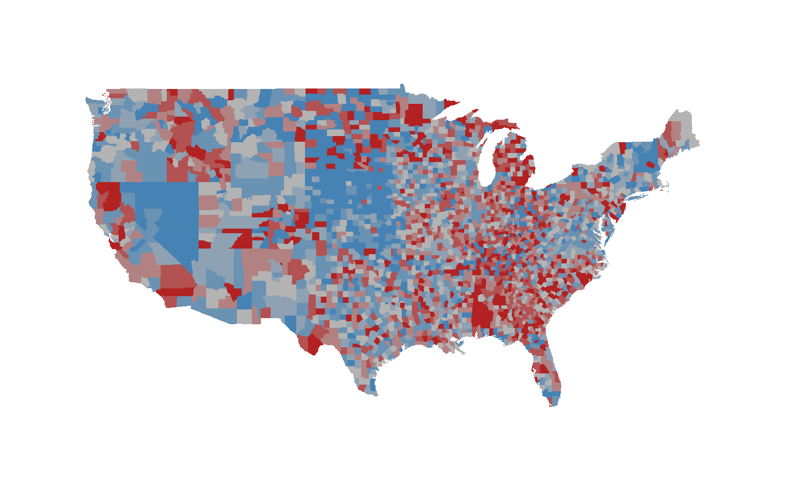

# what went wrong here? 

# our unemployment data (and thus the color vector) follows a different order

cbind( map.id=county.fips$fips, data.id=unemp$fips, color.vector )[ 2500:2510 , ]

      map.id  data.id color.vector
 [1,] "48011" "47149" "#B28282"   
 [2,] "48013" "47151" "#B22222"   
 [3,] "48015" "47153" "#B22222"   
 [4,] "48017" "47155" "#B28282"   
 [5,] "48019" "47157" "#B28282"   
 [6,] "48021" "47159" "#B22222"   
 [7,] "48023" "47161" "#B25252"   
 [8,] "48025" "47163" "#B3B3B3"   
 [9,] "48027" "47165" "#B28282"   
[10,] "48029" "47167" "#B25252"   
[11,] "48031" "47169" "#B25252"

# place the color vector in the correct order

this.order <- match( county.fips$fips, unemp$fips )

color.vec.ordered <- color.vector[ this.order ]

# colors now match their correct counties

map( database="county", col=color.vec.ordered, fill=T, lty=0 )
title( main="Unemployment Levels by County in 2009")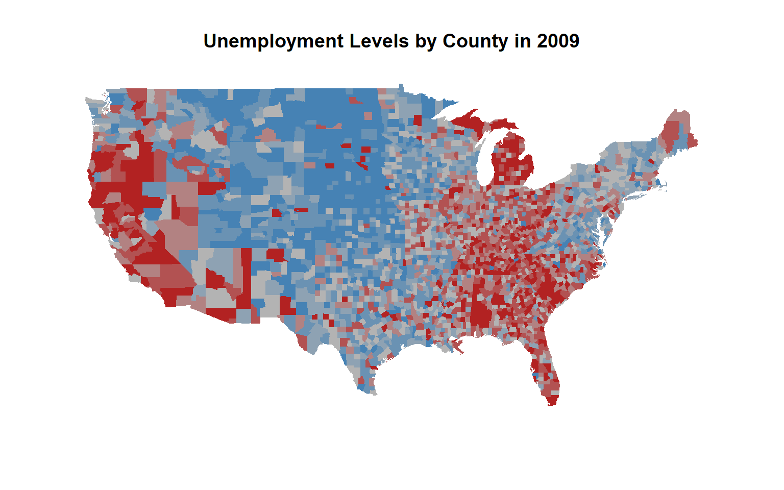

Note that elements can be recycled from your y vector:

x <- c("A","B","C","B")

y <- c("B","D","A","F")

cbind( x, y )

     x   y  
[1,] "A" "B"
[2,] "B" "D"
[3,] "C" "A"
[4,] "B" "F"

match( x, y )

[1]  3  1 NA  1

order.y <- match( x, y )

y.new <- y[ order.y ]

cbind( x, y.new )

     x   y.new
[1,] "A" "A"  
[2,] "B" "B"  
[3,] "C" NA   
[4,] "B" "B"