INTRO TO CENSUS DATA AND MAPPING

Data Practicum Community Analytics

Prof. Anthony Howell

Agenda

  • Working with US Census Data
  • Introduction to Mapping
  • Creating Maps in R (Part 1)
    • w/ tigris & getcensus
  • Creating Maps in R (Part 2)
    • w/ tidycensus

Working with US Census Data

  • Data scientists using R often run into two problems:

    • Understanding what data the Census Bureau publishes.

    • Understanding what R packages on CRAN are available to help with their project.

Intro to Census Data

  • The U.S. Census Bureau is the premier source of data about US people, places and economy.

  • This makes the Bureau a natural source of information for data analysts.

  • The Census Bureau publishes two types of data:
    • demographic and geographic

Demographic Data

  • The Census Bureau conducts over 100 Censuses, Surveys and Programs.

  • You can view the full list of programs here.

  • Top 5 most popular(by API requests):

    1. American Community Survey
    2. Decennial Census of Population and Housing
    3. Population Estimates Program
    4. Survey of Business Owners
    5. International Data Base

American Community Survey (ACS).

  • Info on ancestry, education, income, language, migration, disability, employment, housing
  • Used to allocate government funding, track shifting demographics, plan for emergencies, and learn about local communities.
  • Sent to approximately 295,000 addresses monthly (or 3.5 million per year)
  • largest household survey that the Census Bureau administers

1, 3, 5 year ACS estimates
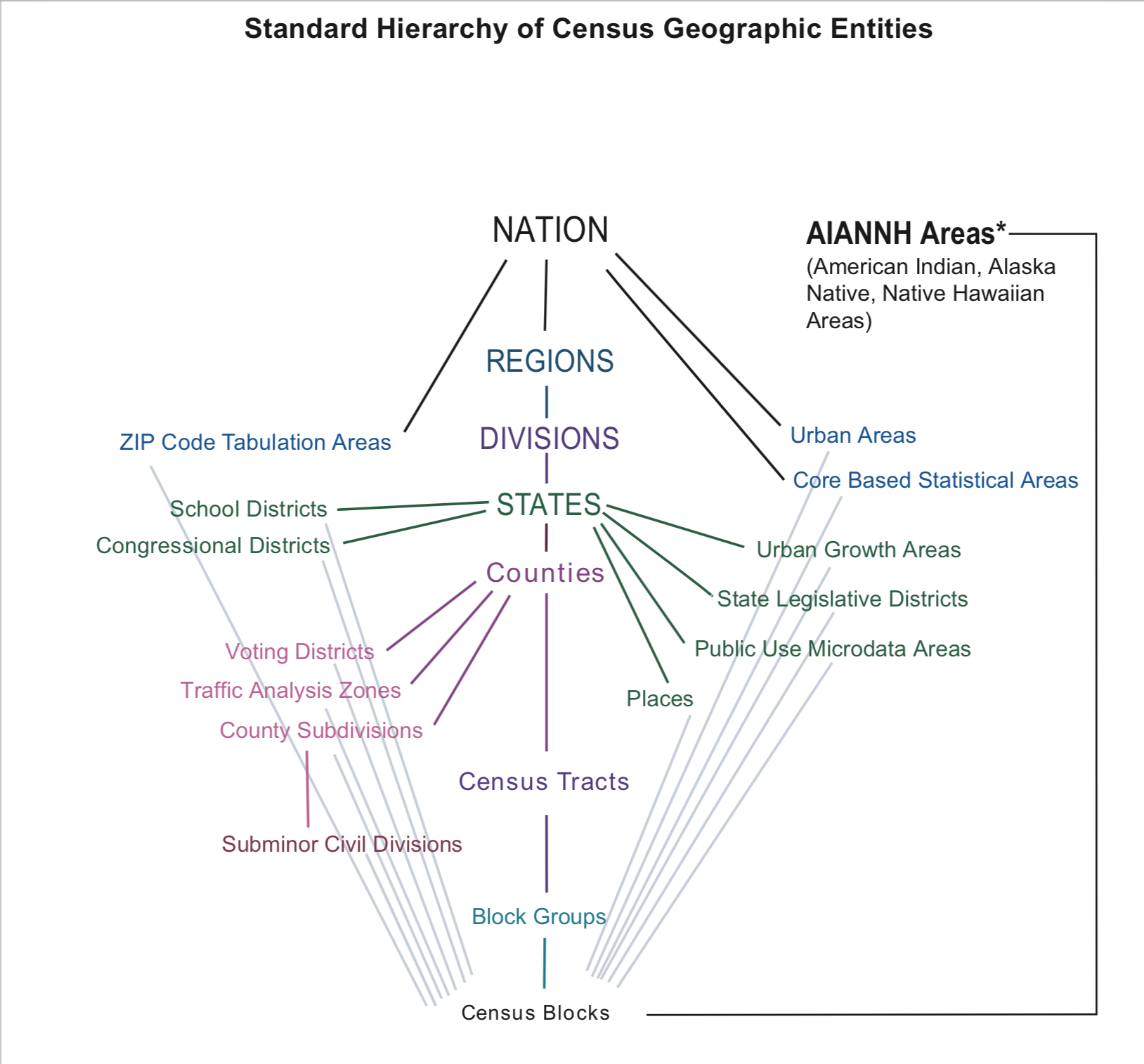
Geographic Data

The Census Bureau’s geographic hierarchy!

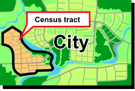
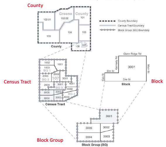
What is a Census Tract?

  • Designed to be relatively homogeneous, e.g. population characteristics, economic status, living conditions

  • Average about 4,000 inhabitants

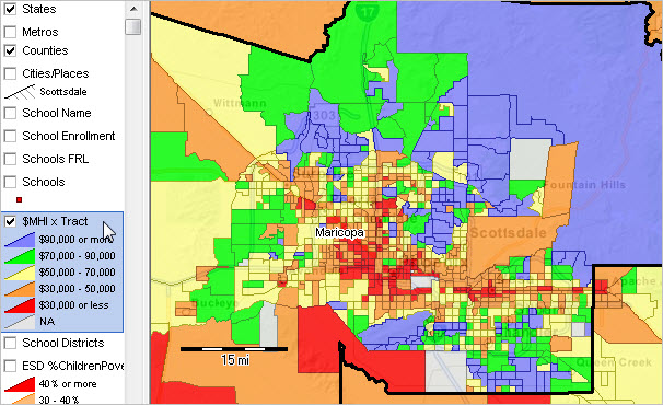
Phoenix Census Tracts

Introduction to Mapping

  • Every house, every tree, every city has its own unique latitude and longitude coordinates.

  • There are two underlying important pieces of information for spatial data:

    • Coordinates of the object (Lat/Long)
    • How the Lat/Long relate to a physical location on Earth
      • Also known as coordinate reference system or CRS

CRS

  • Geographic
    • Uses three-dimensional model of the earth to define specific locations on the surface of the grid
    • longitude (East/West) and latitude (North/South)
  • Projected
    • A translation of the three-dimensional grid onto a two-dimensional plane

CRS

Types of Spatial Data
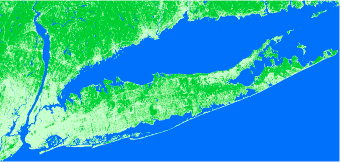
  • Raster
    • Are values within a grid system
    • Example: Satellite imagery
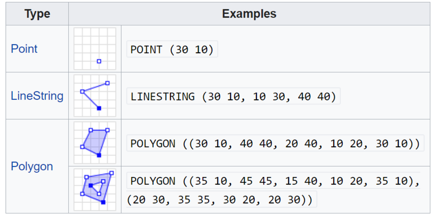
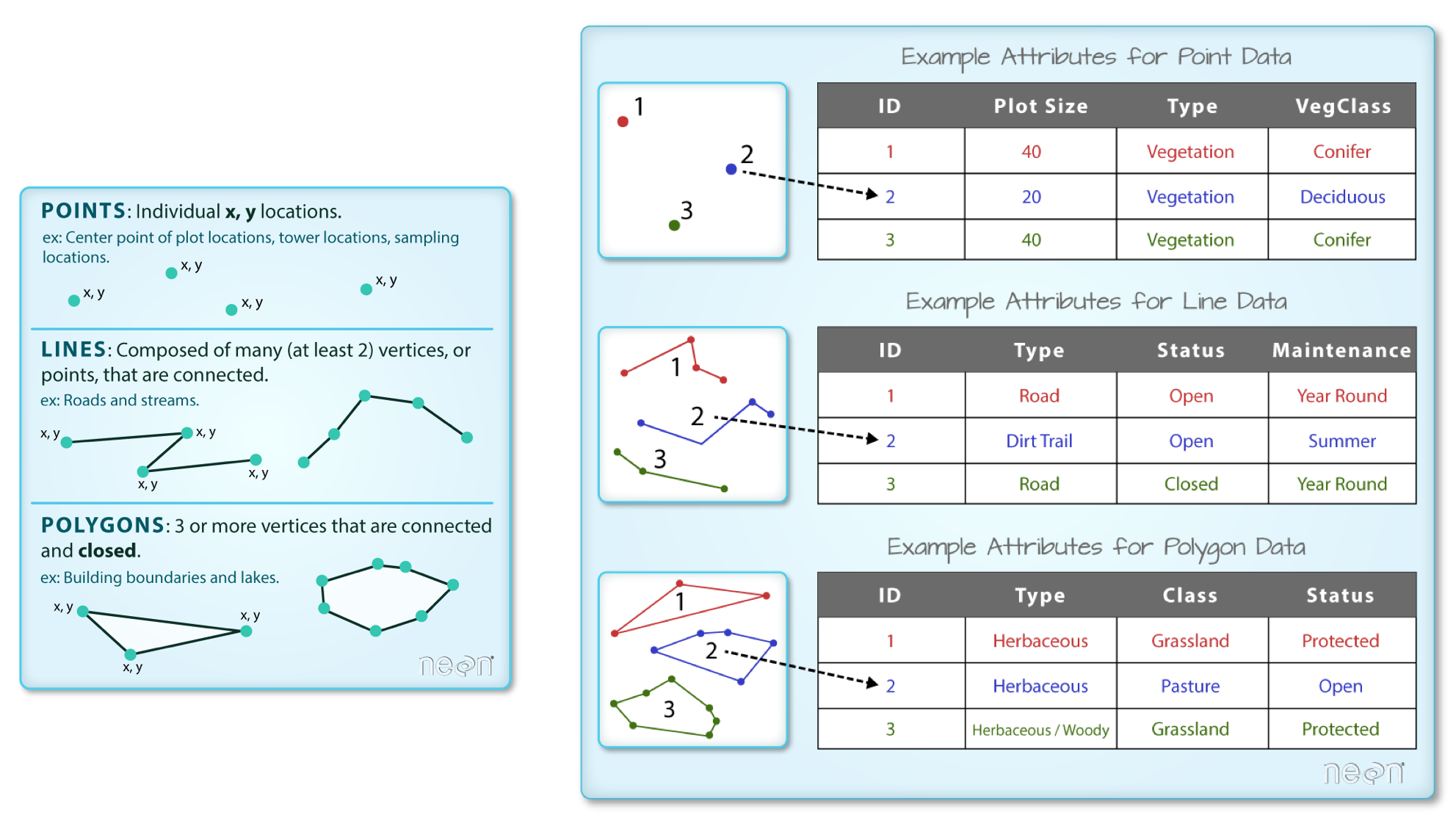
  • Vector
    • Based on points that can be connected to form lines and polygons
    • Located with in a coordinate reference system
    • Example: Road map

Raster

  • Discrete (Land Cover/use maps)
    • Discrete values represent classes, i.e. 1=water; 2=forest
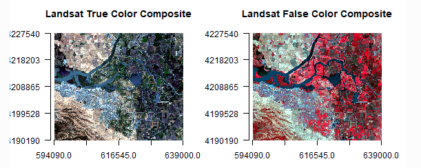
  • Continuous (Satellite Imagery)
    • Grid cells with gradual changing

Vector

Vector (Cont.)

Shape files for Vector

Though we refer to a shape file in the singular, it’s actually a collection of at least three basic files:

  • .shp - lists shape and vertices
  • .shx - has index with offsets
  • .dbf - relationship file between geometry and attributes (data)

All files must be present in the directory and named the same (except for the file extension) to import correctly.

Mapping

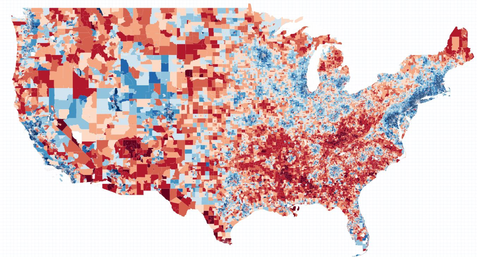
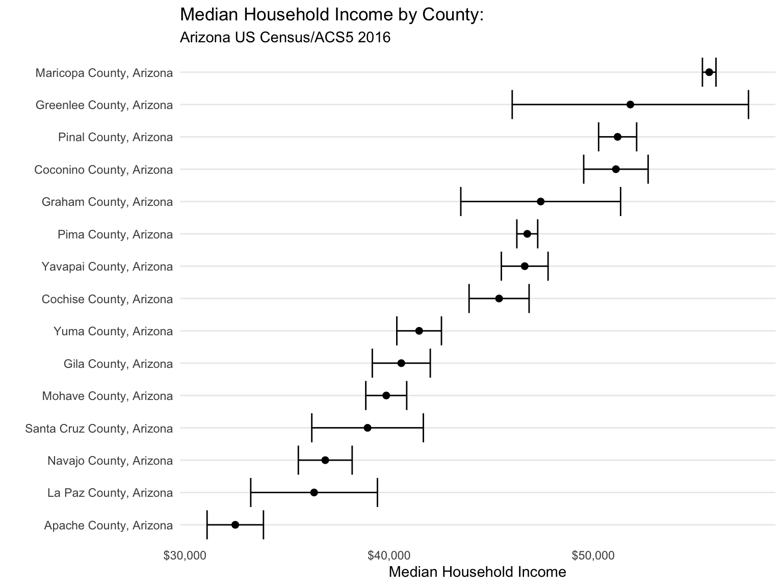
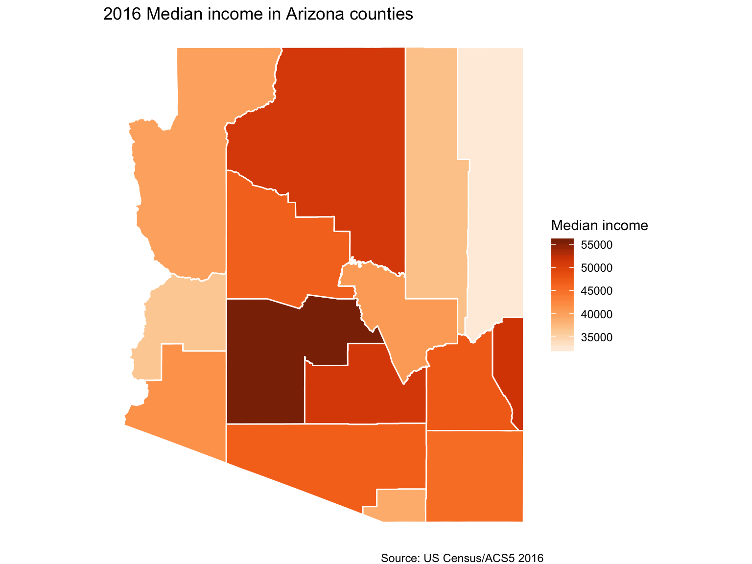
  • Use vector data and shapefiles to create choropleth maps

  • Household Income by Census Tract

Creating Maps in R

  • Download map shapefiles and census data
    • via online downloads (Old School – and it sucks!)
    • via API w/ tigris for maps & getcensus for census data
    • via API w/tidycensus for maps and census data (WINNER!)

Old School Mapping Approach

Old School Mapping Approach

  1. Download data and transform data
    • Excel
  2. Find and download shapefiles
    • Census TIGER
  3. Import maps and join with data and style
    • ArcGIS or QGIS
  4. Export and tweak for style further
    • Tableau, CartoDB, Illustrator

Download Data

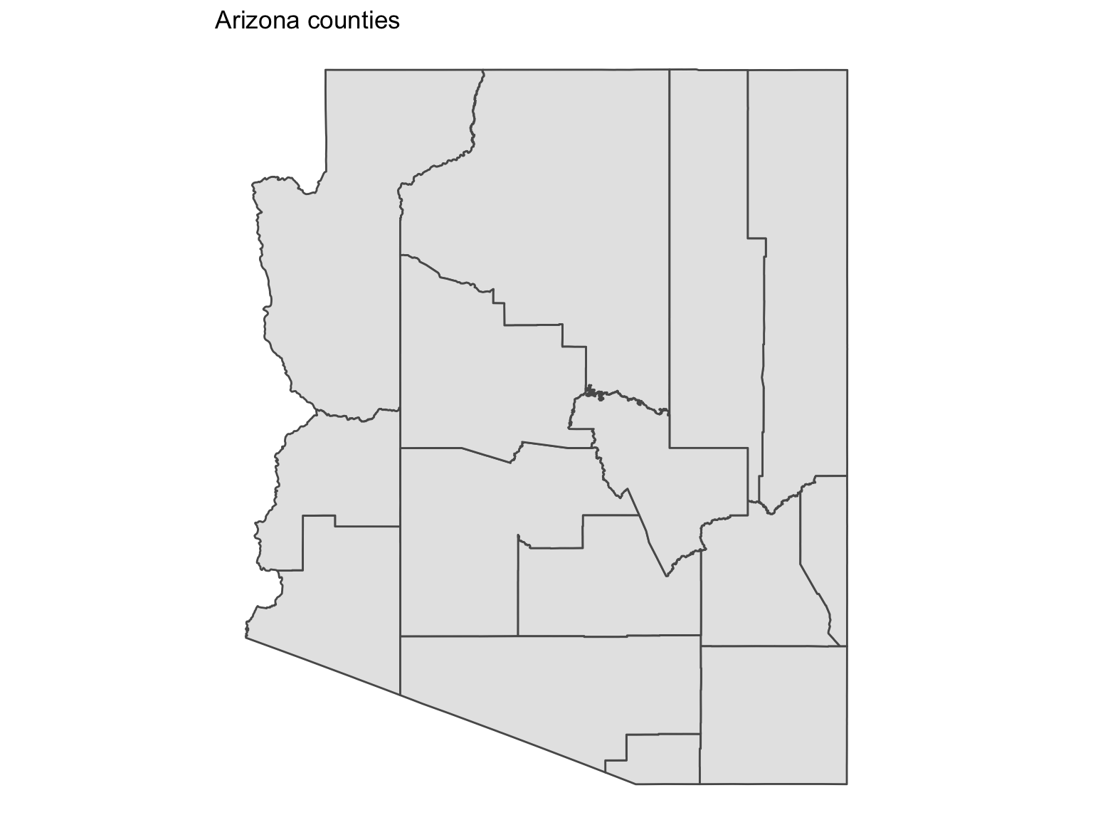
Find and Download Shapefiles

Download a shape file of state boundaries from the Census.

Find downloaded data on computer

Point R (or other spatial software) to correct filepath find File Paths, folders, etc.

  • Time consuming and difficult (esp. for beginners) to even read-in the shapefile and census data to spatial software

New Approach! Downloading shape files directly into R

Using the tigris package, which lets us download Census shapefiles directly into R without having to unzip and point to directories, etc.

Simply call any of these functions (with the proper location variables):

  • tracts()
  • counties()
  • school_districts()
  • roads()

Downloading Census data into R via API

Instead of downloading data from the horrible-to-navigate Census FactFinder or pleasant-to-navigate CensusReporter.org we can pull the code with the censusapi package from Hannah Recht, of Bloomberg.

Load the censusapi library

First, sign up for a census key.

Second, replace YOURKEYHERE with your Census API key.

# Add key to .Renviron
Sys.setenv(CENSUS_KEY="YOURKEYHERE") 
# Check to see that the expected key is output in your R console
Sys.getenv("CENSUS_KEY")

Look up Census tables

Check out the dozens of data sets you can access.

apis <- listCensusApis()
View(apis)

Downloading Census data

We’ll focus on using the getCensus() function from the package. It makes an API call and returns a data frame of results.

These are the arguments you’ll need to pass it:

  • name - the name of the Census data set, like “acs5” or “timeseries/bds/firms”
  • vintage - the year of the data set
  • vars - one or more variables to access
  • region - the geography level of data, like county or tracts or state

Get Census metadata

You can use listCensusMetadata() to see what tables might be available from the ACS Census survey.

acs_vars <- listCensusMetadata(name="acs/acs5", type="variables", vintage=2016)
View(acs_vars)

Slow Process! Please don’t run this right now.

Search for data variable names

In the search finder window, type variable of interest, i.e. median household income

Census variables names

  • B21004_001E, B19013_001M, etc.
    • This is reference to a Census table of information.
    • For example, A14009 is Average Household Income by Race for that polygon of data in that row
    • When you export data from the Census, the variables get translated to this sort of format
    • You’ll have to remember when you download it or look it up.

Downloading median income

##   state county                     NAME B19013_001E B19013_001M
## 1    04    001   Apache County, Arizona       32460        1381
## 2    04    003  Cochise County, Arizona       45383        1470
## 3    04    005 Coconino County, Arizona       51106        1578
## 4    04    007     Gila County, Arizona       40593        1420
## 5    04    009   Graham County, Arizona       47422        3914
## 6    04    011 Greenlee County, Arizona       51813        5787

Data Exploration

Data Exploration

Downloading Arizona Shapefile

First, let’s make sure the shape files download as sf files (because it can also handle sp versions, as well)

If cb is set to TRUE, it downloads a generalized (1:500k) counties file. Default is FALSE (the most detailed TIGER file).

What the az object looks like

View(az)

What are the variables

  • STATEFP is the state fips code.
    • That stands for the Federal Information Processing Standard. It’s a standardized way to identify states, counties, census tracts, etc.
  • GEOID is also part of the fips code.
    • In this instance it’s only two digits wide.
    • The more specific you get into the Census boundaries, the longer the number gets.
  • geometry
    • This is the Coordinate Reference System (CRS) data

Mapping Arizona

Notes on some code

  theme_void() +
  theme(panel.grid.major = element_line(colour = 'transparent')) +
  • theme_void() is a special function that gets rid of grids and gray space for maps
  • theme() is how you can alter specific styles of the visualization
  • theme_void() is a collection of individual theme() modifications

Time to join the map data and median income data

Join Income Data (az_income) and Spatial (az) Map Data

  state county                   NAME B19013_001E B19013_001M
1    04    001 Apache County, Arizona       32460        1381
 [1] "015" "005" "009" "013" "027" "001" "025" "021" "011" "023" "003"
[12] "017" "019" "012" "007"

Did it work?

##  [1] "STATEFP"     "COUNTYFP"    "COUNTYNS"    "AFFGEOID"    "GEOID"      
##  [6] "NAME.x"      "LSAD"        "ALAND"       "AWATER"      "state"      
## [11] "NAME.y"      "B19013_001E" "B19013_001M" "geometry"
## Simple feature collection with 1 feature and 13 fields
## geometry type:  MULTIPOLYGON
## dimension:      XY
## bbox:           xmin: -114.7548 ymin: 34.20963 xmax: -112.5293 ymax: 37.00075
## epsg (SRID):    4269
## proj4string:    +proj=longlat +ellps=GRS80 +towgs84=0,0,0,0,0,0,0 +no_defs
##   STATEFP COUNTYFP COUNTYNS       AFFGEOID GEOID NAME.x LSAD       ALAND
## 1      04      015 00025445 0500000US04015 04015 Mohave   06 34475503964
##      AWATER state                 NAME.y B19013_001E B19013_001M
## 1 387344307    04 Mohave County, Arizona       39856        1002
##                         geometry
## 1 MULTIPOLYGON (((-114.7532 3...

Arizona median income

Download Census data and shapefiles together

Newest package for Census data: tidycensus

With tidycensus, you can download the shape files with the data you want already attached. No joins necessary.

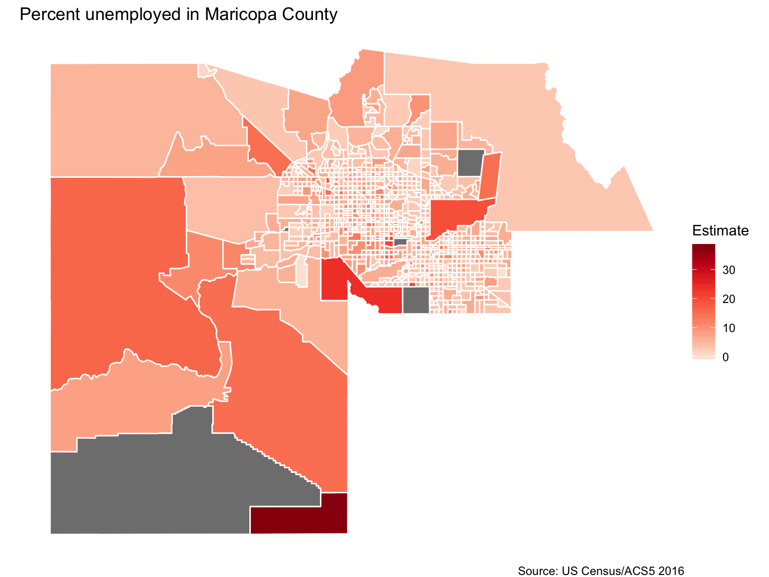
Let’s get right into mapping. We’ll calculate unemployment percents by Census tract in Maricopa County. It’ll involve wrangling some data. But querying the data with get_acs() will be easy and so will getting the shape file by simply passing it geometry=T.

Load up tidycensus

Pass it your Census key.

Search for variables

## # A tibble: 1 x 4
##   name    label                     concept               contains.unemplo…
##   <chr>   <chr>                     <chr>                 <lgl>            
## 1 B12006… ESTIMATE!!TOTAL!!NEVER M… MARITAL STATUS BY SE… TRUE

Search for Variables with View

  • Select Filter (top left). In label box, type Hispanic
  • We want the total non-hispanic population (B03001_002)

Getting unmployment figures

## Simple feature collection with 6 features and 5 fields
## geometry type:  MULTIPOLYGON
## dimension:      XY
## bbox:           xmin: -112.0654 ymin: 33.46573 xmax: -111.04 ymax: 34.03733
## epsg (SRID):    4269
## proj4string:    +proj=longlat +ellps=GRS80 +towgs84=0,0,0,0,0,0,0 +no_defs
##         GEOID                                          NAME   variable
## 1 04013010101 Census Tract 101.01, Maricopa County, Arizona B23025_002
## 2 04013010101 Census Tract 101.01, Maricopa County, Arizona B23025_005
## 3 04013010102 Census Tract 101.02, Maricopa County, Arizona B23025_002
## 4 04013010102 Census Tract 101.02, Maricopa County, Arizona B23025_005
## 5 04013030401 Census Tract 304.01, Maricopa County, Arizona B23025_002
## 6 04013030401 Census Tract 304.01, Maricopa County, Arizona B23025_005
##   estimate moe                       geometry
## 1     1681 333 MULTIPOLYGON (((-111.7869 3...
## 2       87  59 MULTIPOLYGON (((-111.7869 3...
## 3     1767 431 MULTIPOLYGON (((-112.0654 3...
## 4       54  47 MULTIPOLYGON (((-112.0654 3...
## 5     1354 296 MULTIPOLYGON (((-111.9648 3...
## 6       30  49 MULTIPOLYGON (((-111.9648 3...

Transforming the data

head(arizona)

Mapping the data

Faceting maps (Small multiples)

Faceting maps (Small multiples)

head(maricopa)
## Simple feature collection with 6 features and 7 fields
## geometry type:  MULTIPOLYGON
## dimension:      XY
## bbox:           xmin: -112.0654 ymin: 33.46573 xmax: -111.04 ymax: 34.03733
## epsg (SRID):    4269
## proj4string:    +proj=longlat +ellps=GRS80 +towgs84=0,0,0,0,0,0,0 +no_defs
##         GEOID                                          NAME variable
## 1 04013010101 Census Tract 101.01, Maricopa County, Arizona    White
## 2 04013010101 Census Tract 101.01, Maricopa County, Arizona    Black
## 3 04013010101 Census Tract 101.01, Maricopa County, Arizona    Asian
## 4 04013010101 Census Tract 101.01, Maricopa County, Arizona Hispanic
## 5 04013010102 Census Tract 101.02, Maricopa County, Arizona    White
## 6 04013010102 Census Tract 101.02, Maricopa County, Arizona    Black
##   estimate moe summary_est summary_moe                       geometry
## 1     4814 513        4915         517 MULTIPOLYGON (((-111.7869 3...
## 2        0  12        4915         517 MULTIPOLYGON (((-111.7869 3...
## 3       19  33        4915         517 MULTIPOLYGON (((-111.7869 3...
## 4       78 104        4915         517 MULTIPOLYGON (((-111.7869 3...
## 5     4408 592        4602         602 MULTIPOLYGON (((-112.0654 3...
## 6       25  38        4602         602 MULTIPOLYGON (((-112.0654 3...

Transform and map the data

Combine data wrangling and mapping into 1

library(viridis)
maricopa %>%
  mutate(pct = 100 * (estimate / summary_est)) %>%
  ggplot(aes(fill = pct, color = pct)) +
  facet_wrap(~variable) +
  geom_sf() +
  coord_sf(crs = 26915) + 
  scale_fill_viridis(direction=-1) +
  scale_color_viridis(direction=-1) +
  theme_void() +
  theme(panel.grid.major = element_line(colour = 'transparent')) +
  labs(title="Racial geography of Maricopa County, Arizona", caption="Source: US Census 2010")

Transform and map the data

From here, easy to create US maps

Poverty = B17001_002

US County Poverty Map

Lab 2