Counterfactual Analysis
The counterfactual is operationalized by identifying a group that you believe represents what the treatment group would look like if they receive no treatment.
A counterfactual assertion is a conditional whose antecedent is false and whose consequent describes how the world would have been if the antecedent had obtained. The counterfactual takes the form of a subjunctive conditional: “If P had obtained, then Q would have obtained”. In understanding and assessing such a statement we are asked to consider how the world would have been if the antecedent condition had obtained. For example, “If the wind had not reached 50 miles per hour, the bridge would not have collapsed” or “If the Security Council had acted, the war would have been averted.” We can ask two types of questions about counterfactual conditionals: What is the meaning of the statement, and how do we determine whether it is true or false? A counterfactual conditional cannot be evaluated as a truth-functional conditional, since a truth-functional conditional with false antecedent is ipso facto true. (That is, “if P then Q” is equivalent to “either not P or Q”.) So is it necessary to provide a logical analysis of the truth conditions of counterfactuals if they are to be useful in rigorous thought.
There is a close relationship between counterfactual reasoning and causal reasoning. If we assert that “P caused Q (in the circumstances Ci)”, it is implied that we would assert: “If P had not occurred (in circumstances Ci) then Q would not have occurred.” So a causal judgment implies a set of counterfactual judgments. Symmetrically, a counterfactual judgment is commonly supported by reference to one or more causal processes that would have conveyed the world from the situation of the antecedent to the consequent. When we judge that the Tacoma Narrows Bridge would not have collapsed had the wind not reached 50 miles per hour, we rely on a causal theory of the structural dynamics of the bridge and the effects of the wind in reaching the consequent.
How do we assign a truth value to a counterfactual statement? The most systematic answer is to appeal to causal relations and causal laws. If we believe that we have a true causal analysis of the occurrence of Q, and if P is a necessary part of the set of sufficient conditions that bring Q to pass—then we can argue that, had P occurred, Q would have occurred. David Lewis (1973) analyzes the truth conditions and logic of counterfactuals in terms of possible worlds (possible world semantics). A counterfactual is interpreted as a statement about how things occur in other possible worlds governed by the same laws of nature. Roughly: “in every possible world that is relevantly similar to the existing world but in which the wind does not reach 50 miles per hour, the bridge does not collapse.” What constitutes “relevant similarity” between worlds is explained in terms of “being subject to the same laws of nature.” On this approach we understand the counterfactual “If P had occurred, Q would have occurred” as a statement along these lines: “P & {laws of nature} entail Q”. This construction introduces a notion of “physical necessity” to the rendering of counterfactuals: given P, it is physically necessary that Q.
Citations:
Lewis, David K. 1973. Counterfactuals. Cambridge: Harvard University Press.
Encyclopedia of Social Science Research Methods, edited by Michael Lewis-Beck (University of Iowa), Alan Bryman (Loughborough University), and Tim Futing Liao. Sage Publications.
Some Things to Consider:
Lewis was influential in developing a rigorous formulation and language for counterfactual reasoning. Note that he was a philosopher, so he drew heavily upon logic to build a framework, and thus you see emphasis on if-then conditions and truth statements.
Statistical reasoning used in evaluation draws upon probabalistic determinism, which tries to understand probabalistic relationships between events.
Truth statement: If you pay $800 to attend the Kaplan LSAT prep course, you WILL score above a 130 on your LSAT.
Probabalistic statement: If you pay $800 to attend the Kaplan LSAT prep course, the PROBABILITY of scoring above a 130 on the LSAT will increase by X points.
Statisticians use a conditional notation to represent the probabalistic representation of the counterfactual. We write a conditional probability as follows:
Pr( A | B )
This reads as probability that A occurs given that B has occured. Then we augment this notation by incorporating the notion of “how the world would have been if the antecedent had obtained” using an intervention or a “treatment”:
Pr( Y = TRUE | Treatment = TRUE ) - Pr( Y = TRUE | Treatment = FALSE )
Which is to say, the outcome observed in a world where they treatment does not occur represents the baseline reality, and the improvements in the outcome in a world where the treatment was administered can then be causally attributed to the treatment (given a bunch of caveats). The treatment takes the form of the difference between two groups.
The formulation above as Y=TRUE implies that the outcome is discrete - the student got into college, the patient survived the surgery, or the parolee did not return to prison in 12 months.
In cases where the outcome is continuous, such as income levels or wheat yield per acre, the notation would only be slightly different:
[ mean(Y) | Treatment = TRUE ] - [ mean(Y) | Treatment = FALSE ]
Or more succinctly:
Y(t) - Y(c)
The outcome is measured now as a difference of means instead of a change in probabilities of observing success. Thus, we typically care about the Average Treatment Effects because it is the easiest thing to measure (the average outcome for the treatment and control groups) and most succinct way to communicate program effectiveness in evaluation studies.
Important Consideration for Interpretting Impact
The probabalistic nature of causal relationships in social science poses challenges to inference because we will almost always observe some differences in group means. The hard part is determining whether the observed differences are (1) statistically meaningful, i.e. significant, (2) pragmatically meaningful, i.e. large enough effect sizes to warrant investments given a cost-benefit calculation and alternative program models we can fund, and (3) the relationship is causal (think back to the classroom size example where billions were spent reducing class sizes and most schools saw no improvements in test scores).
More so, the marginal nature of program success can pose a challenge to communicating program impact to funders, stakeholders, or the general population. Should we be excited about a 1% increase in an outcome? If we are talking test scores in school, probably not. If we are talking growth in the US economy, that is a huge impact that equates to hundreds of billions of dollars, so yes!
More importantly, if we increase growth by 1% and it is a persistent effect then the benefits will compound over time. This is a very subtle but important consideration in understanding program impact.
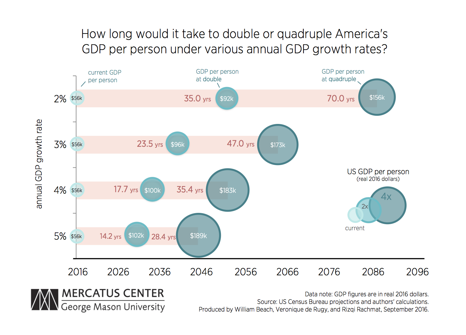
If we observe that the program results in a 10% change the REALLY important question is whether it is a change in a stock of a value or a change in the flow of a value? A change in a stock is a one-time bump in the outcome and a change in a flow compounds over time rather quickly.
For example, if median income is $56,000 then a growth rate of 2% results in a salary of $57k and a growth rate of 5% resuls in a salary of $59k the following year. There is not a huge difference between $57k and $59k so we might be tempted to discount the importance of the intervention that increased the GDP growth rate. HOWEVER, growth compounds annually over time so these small differences are amplified through the magic of exponential growth. The small change in annual growth rates results in huge differences in the size of the economy over time.
For example, when we look at how data analytics can impact the performance of businesses, government agencies, or political campaigns we might see a slight increase in performance such as market or voter share rising from 10% to 15%. On an annual basis the stock measure of market share will not change that much in a single year, but these are annual flows that represent changes to the stock over time. Over several years the aggregate impact can be huge.
This was essentially the story we see in the Good to Great companies popularized by Jim Collins. The high-performing companies were not those taking big risks to introduce new products or splashy mergers. Rather, they were companies that only performed slightly better than the market, but they did so consistently over time by focusing on fundamentals. Those small annual differences quickly compounded into huge market gains for the good to great companies.

We will spend a lot of time this semester looking at program effects, how we can identify them, and how we can contextualize them to understand not just whether our results are statistically significant, but whether they are practically important as well. In each study practice trying to make sense of the practical implications of a program intervention. Does it impact a stock or a flow? Is the effect small or large?
The Importance of the Null Hypothesis
It is important to be conscious of the null hypothesis any time a statistical test is conducted. Use your counterfactual group as the null so that your test for significance will tell you whether the treatment has generated any significant differences in the outcome of interest.
The default in most models is whether the treatment coefficient is different than zero, and that may or may not be a meaningful comparison!
One of the biggest mistakes novice evaluators will make is failing to create a meaningful null hypothesis. As a result, even when statistical models are significant it can be hard to tell whether they say anything meaningful about program impact.
Good impact evaluations share two characteristics:
- The evaluator has been thoughtful about what the ideal counterfactual group looks like in the study.
- The regression model is set up so that results represent a comparison of outcomes between the “treatment” group and its comparison group.
In many cases this is harder than one might think! Especially when the data contains multiple time periods and multiple treatment groups.
For example, if we have a simple study design with randomization and ensures groups are equivalent, and we have a post-treatment measure of outcomes in our study, we can determine the average treatment effect with a simple dummy variable model:
Y = b0 + b1•Treat_Dummy + e
Recall that b0 will capture the average level of Y for the control group (the omitted category), and b1 represents our hypothesis of interest, the gains we observe in the treatment group above and beyond the control group: Y(t) - Y(c). The default null in regression models is always that the slope is equal to zero, so in this case that the group mean Y(t)-Y(c) is equal to zero, i.e. that there is no program effect.
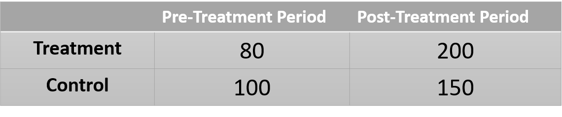
What about the following table of group-level means in a separate study. What regression model do we need to run to determine program impact here?
What is our counterfactual group in this case? How do we capture that group in the model? The result is very clever, but not necessarily obvious. The counterfactual should describe what the world would look like if the treatment group had not received the treatment.
One challenge here is the control group is different than the treatment group, so we cannot just compare the means of the two groups after the program. We are actually going to use the treatment group prior to treatment as the reference. But we know from the control group that we can expect gains independent of the treatment (secular trends). So we create the counterfactual as follows:
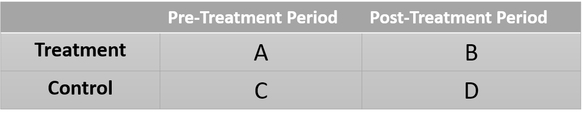
A = pre-treatment group mean
D-C = gains without the treatment
A + (D-C) = state of the world in the absence of a treatment
We can then compare the actual state of the world to our expectd state of the world:
B - [ A + (D-C) ] # best estimate of the treatment effect
Now we have our reasoning worked out. How does this translate into a regression model?
For non-obvious reasons the model described above is written as:
Y = b0 + b1•Treat_Dummy + b2•Time=2_Dummy + b3•Treat_Dummy•Time=2_Dummy + e
We can reconstruct each group mean as follows:
C: b0 = comparison group in time=1
A: b0 + b2 = treatment group in time=1
D: b0 + b2 = control group in time=2
B: b0 + b1 + b2 + b3 = actual group outcome for treatment in time=2
b0 + b1 + b2 = counterfactual group outcome (no treatment effects)
Each coefficient tests the following:
b0: is C different from zero
b1: is the treatment group different from the comparison group in time=1
b2: is there a secular trend in the data
b3: is there a difference between T2 and the counterfactual T2
The coefficient b3 represents the statistical test of the difference between the observed outcome of the treatment group, and the expected outcome for that same group in the absence of the treatment. Which is exactly the test we wanted with exactly the comparison we wanted.
A difference-in-difference framework used to estimate the pay gap during CEO transitions.
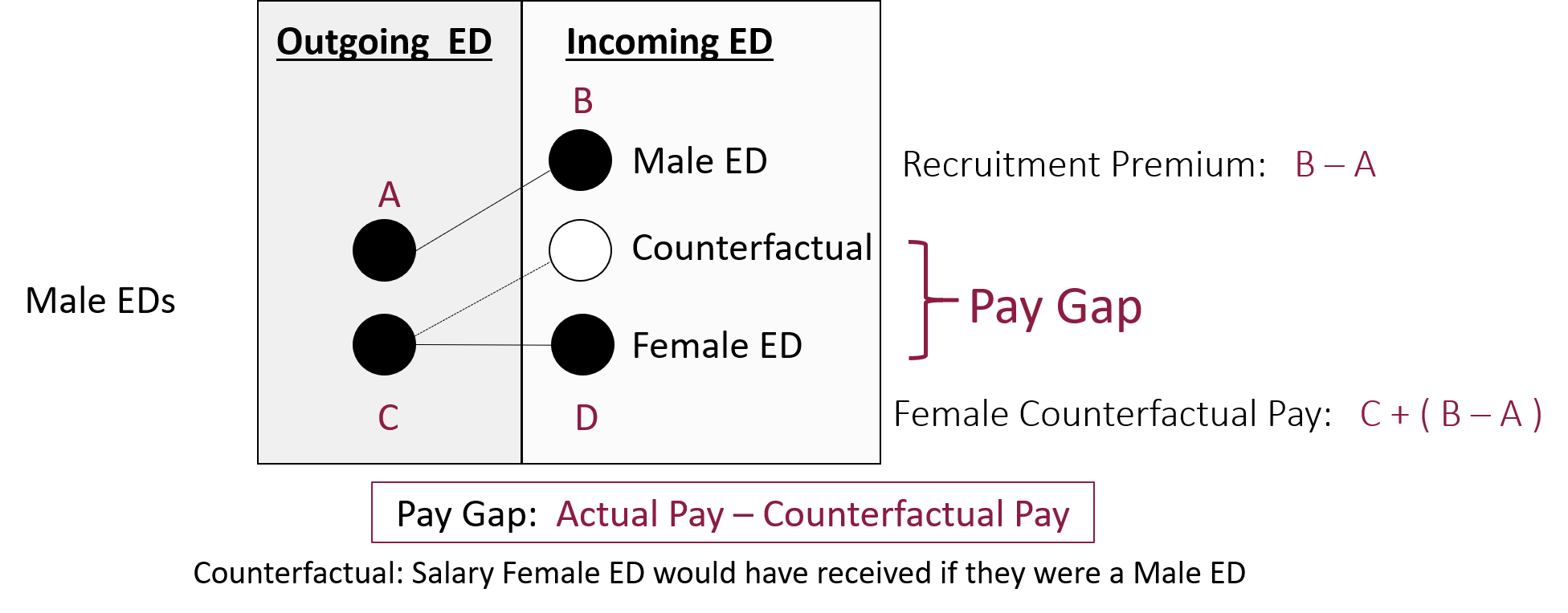
This example is used because before you are familiar with the “difference-in-difference” model it should not be obvious how you go from the 2x2 table to a regression model. If you would run a simple model adding only a dummy variable for the treatment you would get entirely wrong inferences because you are pooling two time periods. If you were to subset the data to remove the first time period then run the model with a dummy for the treatment you would get biased estimates because you are not accounting for pre-treatment differences.
These connundrums are at the heart of counterfactual reasoning, the primary method at the core of inferential statistics. You will get lots of practice with the reasoning component of counterfactual models in Program Eval II (CPP 524) and practice translating from robust reasoning to model specification in Program Eval III (CPP 525).
One of the first known randomizec control trials was described by Sir Ronald Fisher. While socializing with a group a friends a woman made the claim that tea always tastes better when the tea is poured into the milk rather than when milk is poured into the tea. At first blush there is no rational basis for this claim, so many in the group were rightly skeptical and believed it was psychological effect. Fisher, a rising star in statistics, quickly devised a way to test whether she could actually differentiate between the two conditions by having her taste 8 cups of tea, four of which has been prepared by pouring the milk into the tea, and four by pouring the tea into the milk. The preparation was done out of sight so she was left to rely on the taste of the tea only to guess which were which.
The question is, what is the null hypothesis in this experiment?
We would be naive to assume that if there is in fact no difference in taste that she will guess all 8 incorrectly. Since there are only two options for each cup she is almost certain to guess some of them correctly by pure chance. So how do we describe the state of the world where the taste of the tea is the same no matter which method is used to prepare it? How many does she need to get correct before we know that the outcome is unlikely driven by luck?
Read the following description of the problem set-up: The Lady Tasting Tea
Consider a slightly easier problem. A friend tells you that he is psychic and can use his mind to see what is behind walls. You just so happen to be watching Let’s Make a Deal, and they are playing the game with 3 doors that hide 2 goats and 1 car. The contestant picks a door and wins the prize behind it.

If your friend correctly guesses the position of the car in the first round, what is the likelihood of that happening by chance? He has a one in three chance of guessing by luck on the first try.
Pr( selected door = car ) = 0.33
So there is a 33% chance he is delusional but able to fool people.
What about guessing two cars in a row?
Pr( door = car : round 1 ) & Pr( door = car: round 2 ) = (0.33)(0.33) = 0.11
Three cars in a row?
(0.33)(0.33)(0.33) = 0.037
At what point will you be convinced that he is psychic (or at least a good cheater)? How rare does the event need to be to provide sufficient evidence?
What do we expect the typical state of the world to be if he is not psychic? What happens if after five rounds he has guessed correctly four times and incorrectly one time? Is that enough evidence to prove his psychic abilities make him a better guesser than chance? What if it were forty times out of fifty? Does that change our response?
What if there are only two doors and he guesses correctly three times in a row?
(0.5)(0.5)(0.5) = 0.125
There is now a 13% chance of observing that outcome instead of a 4% chance in the case with three doors and three correct guesses. Does that change our view?
The important insight is that when we expect that a program has no impact, or when a claim is false, we would not expect that the control group then outperform the treatment group, or that the treatment group would never do better than the control group. In most cases the null hypothesis represents a distribution of expected outcomes in the absence of an effective program.
Once we have selected a confidence level (our tolerance for a Type II error) the statistical test should tell us the critical value that will differentiate luck from meaningful differences.
When describing the state of the world where the treatment doesn’t matter (tea tastes the same no matter which way you mix the milk) it is more likely that we observe some number of successes that occur by chance (2 out of 8 correct) than no successes at all. Experiments are not as simple as, if she can’t really tell the difference she won’t get any correct.
We must convert our counterfactual view of the world into a meaningful null hypothesis that describes a set of outcomes that fail to support our theory of interest (the program works) and a set of outcomes that supports our theory (those unlikely to occur through chance if the program has no impact).
More generally we need to think about what patterns in data we expect to see if the program is having an impact, and what patterns we expect to see if it is not. Having these things in mind will help you identify the best models that capture your research question most precisely.
Statistical Power Calculator
The NHST (Null Hypothesis Statistical Test) Ritual
- alpha, the criteria used for rejecting the null (0.05) predicts the rate of Type I Errors in repeated samples
- beta ( 1 - power ) predicts the rate of Type II Errors in repeated samples
- effect size for a t-test (Cohen’s d) tells you the distance between the observed population mean and the null
Note that increasing the sample size is unambiguously good in that it lowers Type I and Type II Errors, though there are always real economic costs of the sample in a study.
Similarly, a larger effect size is always better. If you have a very large effect it is easy to detect statistically even with a small sample. As a rule of thumb when looking at Cohen’s d in t-tests:
- 0.2 is a small effect
- 0.5 is a moderate-sized effect
- 0.8 is a large effect
These heuristics on magnitude vary by the type of statistical model (and thus the statistic used to report effect size):
Effect Size Magnitude by Statistic
You determine the effect size for a power calculation by looking at previous research in the domain and using reported statistics to calculate the effect size, or if you are lucky a published meta-analysis will have done this for you already for a lot of studies and you can use the average effect size reported.
When Type I Error appears as 0% it just means it is less than 0.005 and the dashboard rounds the value (it is never actually zero).
Most studies use an alpha of 0.05 and beta of 0.80 because these values balance the trade-off between the two error rates. If one type of error is more costly in your context consider adjusting these while doing a power calculation.
The Strength of Evidence
CPP 524 is a course on research design. It might sound either straight-forward (you just create a treatment and control group and call it a day), or tedious. I suspect that by the end of the semester you will find the topic to be quite fun if you approach it the right way.
Research design and external review of other’s research design can in fact be quite tedious because there are a lot of details to keep track of. You will always have deficiencies in research design that prevent you from being 100% certain the results can be trusted, and it can be mentally taxing to weigh the evidence and decide whether you buy the results.
Not all evaluations are the same. Some provide robust and trustworthy estimates of program impact, and some provide noisy and indeterminate statistics where it is unclear what they actually represent. Whereas last semester we learned about using regression models to estimate the size of a slope, this course is meant to help you develop a qualitative notion of the strength of evidence.
Statistical signifance tells us the likelihood that the model slope differs from the model null, but it does not tell us if the null is a reasonable counterfactual and adequate steps have been taken to remove bias in the slope. Those both occur at the design phase, not the at the point of model estimation.
Internal Validity as a Murder Mystery
Internal validity is the term we use to measure whether our research design sufficient to say with confidence that changes we observe in the data are a result of the program only. In other words, having strong internal validity requires that we must eliminate all of the other salient competing hypotheses that offer an alternative explanation to the observed changes in the data.
We can treat this exercise as a murder mystery. Who created the changes in the data? Our leading theory is that the program did it, but we also must eliminate all of the other suspects.
We will use a check-list approach that we call a Campbell Score, which is a list of the ten most common competing hypotheses that weaken internal validity. We will use the check-list to practice reading research critically to look for holes in design. You will also use the tool to create a research design for a program of your choice, and think through which competing explanations you need to neutralize if you want your results to be compelling.