** Review
*** { @unit = “”, @title = “Overview of the Program Evaluation”, @lecture, @foldout }
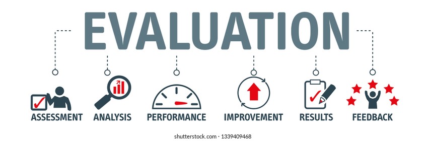
Evidence-Based Practices

What does it mean to live in an evidence-based world? How do we become more data-driven?
It turns out that using data to improve decision-making and organizatoinal performance is not a trivial affair because of a little problem called omitted variable bias (correlation does not equal causation). As a result, we need to combine judicious analytical techniques with feasible approaches to research design in order to understand causal impact of social programs.
Here is a great introduction to a case study that uses evaluation to better understant the impact of a government program by getting past anecdotes to measure program impact.
Understanding Causal Impact Without Randomized Control Trials
In most cases we don’t have resources for large-scale Randomized Control Studies. They typically cost millions of dollars, are sometime unethical, and are often times not feasible. For example, does free trade prevent war? How do you randomized free trade across countries?
Statistics and econometricians have spent 75 years developing powerful regression tools that can be used with observational data and clever quasi-experimental research designs to tease out program impact when RCT’s are not possible. The courses in the Foundations of Program Evaluation sequence build the tools to deploy these methods.
- Foundations of Eval I covers the mechanics of regression.
- Foundations of Eval II covers counterfactual analysis and quasi-experimental approaches to research design.
- Foundations of Eval III covers seven regression models used in causal analysis (for example, interrupted time series).
Let’s start with a simple example. Is caffeine good for you?
What evidence is used to create these assertions? [ link ]
Can you conduct a Randomized Control Trial to study the effects of caffeine on mental health over a long period of time? Is this correlation or causation?
How can we be sure we are measuring the causal impact of coffee on health?
Why is evidence-based management hard?
Just listen to this summary of current knowledge on the topic, then try to succinctly translate it to a rule of thumb physicians should use on whether to recommend coffee to patients.
*** { @unit = “”, @title = “Useful Background Reading”, @reading, @foldout }
Program Impact
This course provides foundational skills in quantitative program evaluation:
Reichardt, C. S., & Bormann, C. A. (1994). Using regression models to estimate program effects. Handbook of practical program evaluation, 417-455. [ pdf ]
The Broader Field of Evaluation
Program evaluation is a large field that deploys a diversity of methodologies beyond quantitative modeling and impact analysis. We focus heavily on the quantitative skills in the Foundations of Eval I, II, and III in this program because data is hard to use, so you need several courses to build a skill set. Qualitative and case-study approaches build from the same foundations in research design, so you can more fully develop some of those skills drawing from knowledge of formal modeling and inference.
For some useful context on evaluation as a field, this short (6-page overview) is helpful:
McNamara, C. (2008). Basic guide to program evaluation. Free Management Library. [ pdf ]
And to get a flavor for debates around approaches to measuring program impact in evaluation:
White, H. (2010). A contribution to current debates in impact evaluation. Evaluation, 16(2), 153-164. [ pdf ]
** Week 1 - Counterfactual Analysis
*** { @unit = “”, @title = “Unit Overview”, @reading, @foldout }
Description
This section provides introduces the concept of a counterfactual reasoning. Key terms include:
- randomized control trials (RCTs)
- average treatment effects
- internal validity
- null hypothesis
Learning Objectives
Once you have completed this section you will be able to identify and
Lab Preview
For Lab-01 you will read an example of a Randomized Control Trial used to study a nutrition and early childhood education program in Columbia. The lab asks for you to report on features of the research design and identify core concepts in the study:
- The control group
- The program theory
- The treatment
- Treatment versus study time-frames
- Confounding factors
Bingham, R., & Felbinger, C. (2002). Evaluation in practice: A methodological approach. CQ Press.
- CH-05: Improving Cognitive Ability in Chronically Deprived Children [pdf]
*** { @unit = “”, @title = “Required Reading”, @reading, @foldout }
Assigned and Recommended Articles or Chapters
Required:
Gertler, P. J., Martinez, S., Premand, P., Rawlings, L. B., & Vermeersch, C. M. (2016). Impact evaluation in practice. The World Bank. [pdf]
- Chapter 3. Causal Inference and Counterfactuals
- Chapter 4. Randomized Selection Methods
For reference:
Reichardt, C. S., & Bormann, C. A. (1994). Using regression models to estimate program effects. Handbook of practical program evaluation, 417-455. [ pdf ]
*** { @unit = “”, @title = “Counterfactual Reasoning”, @lecture, @foldout }
Counterfactual Analysis
A counterfactual assertion is a conditional whose antecedent is false and whose consequent describes how the world would have been if the antecedent had obtained. The counterfactual takes the form of a subjunctive conditional: “If P had obtained, then Q would have obtained”. In understanding and assessing such a statement we are asked to consider how the world would have been if the antecedent condition had obtained. For example, “If the wind had not reached 50 miles per hour, the bridge would not have collapsed” or “If the Security Council had acted, the war would have been averted.” We can ask two types of questions about counterfactual conditionals: What is the meaning of the statement, and how do we determine whether it is true or false? A counterfactual conditional cannot be evaluated as a truth-functional conditional, since a truth-functional conditional with false antecedent is ipso facto true. (That is, “if P then Q” is equivalent to “either not P or Q”.) So is it necessary to provide a logical analysis of the truth conditions of counterfactuals if they are to be useful in rigorous thought.
There is a close relationship between counterfactual reasoning and causal reasoning. If we assert that “P caused Q (in the circumstances Ci)”, it is implied that we would assert: “If P had not occurred (in circumstances Ci) then Q would not have occurred.” So a causal judgment implies a set of counterfactual judgments. Symmetrically, a counterfactual judgment is commonly supported by reference to one or more causal processes that would have conveyed the world from the situation of the antecedent to the consequent. When we judge that the Tacoma Narrows Bridge would not have collapsed had the wind not reached 50 miles per hour, we rely on a causal theory of the structural dynamics of the bridge and the effects of the wind in reaching the consequent.
How do we assign a truth value to a counterfactual statement? The most systematic answer is to appeal to causal relations and causal laws. If we believe that we have a true causal analysis of the occurrence of Q, and if P is a necessary part of the set of sufficient conditions that bring Q to pass—then we can argue that, had P occurred, Q would have occurred. David Lewis (1973) analyzes the truth conditions and logic of counterfactuals in terms of possible worlds (possible world semantics). A counterfactual is interpreted as a statement about how things occur in other possible worlds governed by the same laws of nature. Roughly: “in every possible world that is relevantly similar to the existing world but in which the wind does not reach 50 miles per hour, the bridge does not collapse.” What constitutes “relevant similarity” between worlds is explained in terms of “being subject to the same laws of nature.” On this approach we understand the counterfactual “If P had occurred, Q would have occurred” as a statement along these lines: “P & {laws of nature} entail Q”. This construction introduces a notion of “physical necessity” to the rendering of counterfactuals: given P, it is physically necessary that Q.
Citations:
Lewis, David K. 1973. Counterfactuals. Cambridge: Harvard University Press.
Encyclopedia of Social Science Research Methods, edited by Michael Lewis-Beck (University of Iowa), Alan Bryman (Loughborough University), and Tim Futing Liao. Sage Publications.
Some Things to Consider:
Lewis was influential in developing a rigorous formulation and language for counterfactual reasoning. Note that he was a philosopher, so he drew heavily upon logic to build a framework, and thus you see emphasis on if-then conditions and truth statements.
Statistical reasoning used in evaluation draws upon probabalistic determinism, which tries to understand probabalistic relationships between events.
Truth statement: If you pay $800 to attend the Kaplan LSAT prep course, you WILL score above a 130 on your LSAT.
Probabalistic statement: If you pay $800 to attend the Kaplan LSAT prep course, the PROBABILITY of scoring above a 130 on the LSAT will increase by X points.
Statisticians use a conditional notation to represent the probabalistic representation of the counterfactual. We write a conditional probability as follows:
Pr( A | B )
This reads as probability that A occurs given that B has occured. Then we augment this notation by incorporating the notion of “how the world would have been if the antecedent had obtained” using an intervention or a “treatment”:
Pr( Y = TRUE | Treatment = TRUE ) - Pr( Y = TRUE | Treatment = FALSE )
Which is to say, the outcome observed in a world where they treatment does not occur represents the baseline reality, and the improvements in the outcome in a world where the treatment was administered can then be causally attributed to the treatment (given a bunch of caveats). The treatment takes the form of the difference between two groups.
The formulation above as Y=TRUE implies that the outcome is discrete - the student got into college, the patient survived the surgery, or the parolee did not return to prison in 12 months.
In cases where the outcome is continuous, such as income levels or wheat yield per acre, the notation would only be slightly different:
[ mean(Y) | Treatment = TRUE ] - [ mean(Y) | Treatment = FALSE ]
Or more succinctly:
Y(t) - Y(c)
The outcome is measured now as a difference of means instead of a change in probabilities of observing success. Thus, we typically care about the Average Treatment Effects because it is the easiest thing to measure (the average outcome for the treatment and control groups) and most succinct way to communicate program effectiveness in evaluation studies.
The probabalistic nature of causal relationships in social science poses challenges to inference because we will almost always observe some differences in group means. The hard part is determining whether the observed differences are (1) statistically meaningful, i.e. significant, (2) pragmatically meaningful, i.e. large enough effect sizes to warrant investments given a cost-benefit calculation and alternative program models we can fund, and (3) the relationship is causal (think back to the classroom size example where billions were spent reducing class sizes and most schools saw no improvements in test scores).
More so, the marginal nature of program success can pose a challenge to communicating program impact to funders, stakeholders, or the general population. Should we be excited about a 1% increase in an outcome? If we are talking test scores in school, probably not. If we are talking growth in the US economy, that is a huge impact that equates to hundreds of billions of dollars, so yes!
More so, if we observe that the program results in a 10% change the REALLY important question is whether it is a change in a stock of a value or a flow of a value? This difference radically changes the interpretation of a model coefficient because a change in a stock is a one-time bump and a change in a flow compounds over time rather quickly:
For example, when we look at how data analytics can be used to “moneyball” businesses, political campaigns and government we find that things like predicting a profitable new product can result in short-term gains in market share (a stock measure). Investments in data warehouse capacity and building data-driven management practices can impact efficiency and rates of growth, thus compounding benefits over time. This was essentially the story we see in the Good to Great companies popularized by Jim Collins.

We will spend a lot of time this semester looking at program effects, how we can identify them, and how we can contextualize them to understand not just whether our results are statistically significant, but whether they are practically important as well.
*** { @unit = “”, @title = “Null Hypotheses”, @lecture, @foldout }
The Importance of the Null Hypothesis
One of the biggest mistakes novice evaluators will make is failing to create a meaningful null hypothesis. As a result, even when statistical models are significant it can be hard to tell whether they say anything meaningful about program impact.
Good impact evaluations share two characteristics:
- The evaluator has been thoughtful about what the ideal counterfactual group looks like in the study.
- The regression model is set up so that results represent a comparison of outcomes between the “treatment” group and its comparison group.
In many cases this is harder than one might think! Especially when the data contains multiple time periods and multiple treatment groups.
For example, if we have a simple study design with randomization and ensures groups are equivalent, and we have a post-treatment measure of outcomes in our study, we can determine the average treatment effect with a simple dummy variable model:
Y = b0 + b1•Treat_Dummy + e
Recall that b0 will capture the average level of Y for the control group (the omitted category), and b1 represents our hypothesis of interest, the gains we observe in the treatment group above and beyond the control group: Y(t) - Y(c). The default null in regression models is always that the slope is equal to zero, so in this case that the group mean Y(t)-Y(c) is equal to zero, i.e. that there is no program effect.
What about the following table of group-level means in a separate study. What regression model do we need to run to determine program impact here?
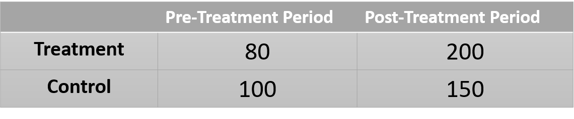
What is our counterfactual group in this case? How do we capture that group in the model? The result is very clever, but not necessarily obvious. The counterfactual should describe what the world would look like if the treatment group had not received the treatment.
One challenge here is the control group is different than the treatment group, so we cannot just compare the means of the two groups after the program. We are actually going to use the treatment group prior to treatment as the reference. But we know from the control group that we can expect gains independent of the treatment (secular trends). So we create the counterfactual as follows:
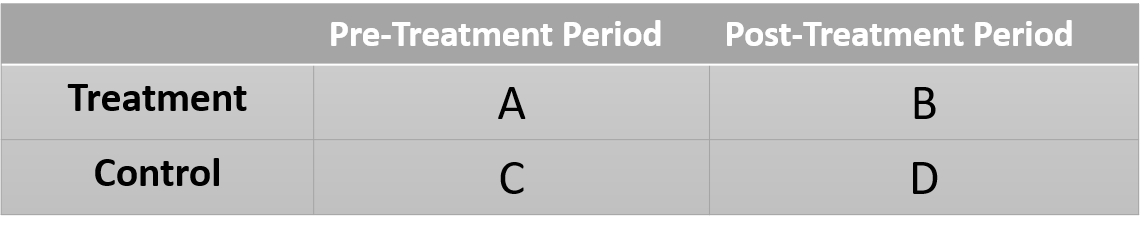
A = pre-treatment group mean
D-C = gains without the treatment
A + (D-C) = state of the world in the absence of a treatment
We can then compare the actual state of the world to our expectd state of the world:
B - [ A + (D-C) ] # best estimate of the treatment effect
Now we have our reasoning worked out. How does this translate into a regression model?
For non-obvious reasons the model described above is written as:
Y = b0 + b1•Treat_Dummy + b2•Time=2_Dummy + b3•Treat_Dummy•Time=2_Dummy + e
We can reconstruct each group mean as follows:
C: b0 = comparison group in time=1
A: b0 + b2 = treatment group in time=1
D: b0 + b2 = control group in time=2
B: b0 + b1 + b2 + b3 = actual group outcome for treatment in time=2
b0 + b1 + b2 = counterfactual group outcome (no treatment effects)
Each coefficient tests the following:
b0: is C different from zero
b1: is the treatment group different from the comparison group in time=1
b2: is there a secular trend in the data
b3: is there a difference between T2 and the counterfactual T2
The coefficient b3 represents the statistical test of the difference between the observed outcome of the treatment group, and the expected outcome for that same group in the absence of the treatment. Which is exactly the test we wanted with exactly the comparison we wanted.
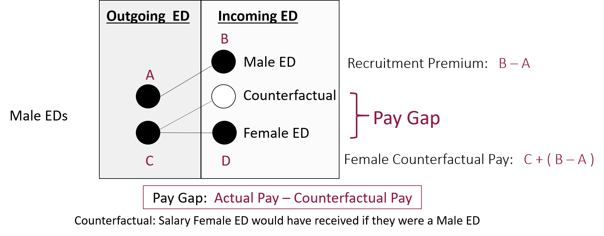
A difference-in-difference framework used to estimate the pay gap during CEO transitions.
This example is used because before you are familiar with the “difference-in-difference” model it should not be obvious how you go from the 2x2 table to a regression model. If you would run a simple model adding only a dummy variable for the treatment you would get entirely wrong inferences because you are pooling two time periods. If you were to subset the data to remove the first time period then run the model with a dummy for the treatment you would get biased estimates because you are not accounting for pre-treatment differences.
These connundrums are at the heart of counterfactual reasoning, the primary method at the core of inferential statistics. You will get lots of practice with the reasoning component of counterfactual models in Program Eval II (CPP 524) and practice translating from robust reasoning to model specification in Program Eval III (CPP 525).
One of the first known randomizec control trials was described by Sir Ronald Fisher. While socializing with a group a friends a woman made the claim that tea always tastes better when the tea is poured into the milk rather than when milk is poured into the tea. At first blush there is no rational basis for this claim, so many in the group were rightly skeptical and believed it was psychological effect. Fisher, a rising star in statistics, quickly devised a way to test whether she could actually differentiate between the two conditions by having her taste 8 cups of tea, four of which has been prepared by pouring the milk into the tea, and four by pouring the tea into the milk. The preparation was done out of sight so she was left to rely on the taste of the tea only to guess which were which.
The question is, what is the null hypothesis in this experiment?
We would be naive to assume that if there is in fact no difference in taste that she will guess all 8 incorrectly. Since there are only two options for each cup she is almost certain to guess some of them correctly by pure chance. So how do we describe the state of the world where the taste of the tea is the same no matter which method is used to prepare it? How many does she need to get correct before we know that the outcome is unlikely driven by luck?
Read the following description of the problem set-up: The Lady Tasting Tea
Consider a slightly easier problem. A friend tells you that he is psychic and can use his mind to see what is behind walls. You just so happen to be watching Let’s Make a Deal, and they are playing the game with 3 doors that hide 2 goats and 1 car. The contestant picks a door and wins the prize behind it.

If your friend correctly guesses the position of the car in the first round, what is the likelihood of that happening by chance? He has a one in three chance of guessing by luck on the first try.
Pr( selected door = car ) = 0.33
So there is a 33% chance he is delusional but able to fool people.
What about guessing two cars in a row?
Pr( door = car : round 1 ) & Pr( door = car: round 2 ) = (0.33)(0.33) = 0.11
Three cars in a row?
(0.33)(0.33)(0.33) = 0.037
At what point will you be convinced that he is psychic (or at least a good cheater)? How rare does the event need to be to provide sufficient evidence?
What do we expect the typical state of the world to be if he is not psychic? What happens if after five rounds he has guessed correctly four times and incorrectly one time? Is that enough evidence to prove his psychic abilities make him a better guesser than chance? What if it were forty times out of fifty? Does that change our response?
What if there are only two doors and he guesses correctly three times in a row?
(0.5)(0.5)(0.5) = 0.125
There is now a 13% chance of observing that outcome instead of a 4% chance in the case with three doors and three correct guesses. Does that change our view?
The important insight is that when we expect that a program has no impact, or when a claim is false, we would not expect that the control group then outperform the treatment group, or that the treatment group would never do better than the control group. In most cases the null hypothesis represents a distribution of expected outcomes in the absence of an effective program.
Once we have selected a confidence level (our tolerance for a Type II error) the statistical test should tell us the critical value that will differentiate luck from meaningful differences.
When describing the state of the world where the treatment doesn’t matter (tea tastes the same no matter which way you mix the milk) it is more likely that we observe some number of successes that occur by chance (2 out of 8 correct) than no successes at all. Experiments are not as simple as, if she can’t really tell the difference she won’t get any correct.
We must convert our counterfactual view of the world into a meaningful null hypothesis that describes a set of outcomes that fail to support our theory of interest (the program works) and a set of outcomes that supports our theory (those unlikely to occur through chance if the program has no impact).
More generally we need to think about what patterns in data we expect to see if the program is having an impact, and what patterns we expect to see if it is not. Having these things in mind will help you identify the best models that capture your research question most precisely.
*** { @unit = “”, @title = “Statistical Power”, @reading, @foldout }
Statistical Power Calculator
The NHST (Null Hypothesis Statistical Test) Ritual
- alpha, the criteria used for rejecting the null (0.05) predicts the rate of Type I Errors in repeated samples
- beta ( 1 - power ) predicts the rate of Type II Errors in repeated samples
- effect size for a t-test (Cohen’s d) tells you the distance between the observed population mean and the null
Note that increasing the sample size is unambiguously good in that it lowers Type I and Type II Errors, though there are always real economic costs of the sample in a study.
Similarly, a larger effect size is always better. If you have a very large effect it is easy to detect statistically even with a small sample. As a rule of thumb when looking at Cohen’s d in t-tests:
- 0.2 is a small effect
- 0.5 is a moderate-sized effect
- 0.8 is a large effect
These heuristics on magnitude vary by the type of statistical model (and thus the statistic used to report effect size):
Effect Size Magnitude by Statistic
You determine the effect size for a power calculation by looking at previous research in the domain and using reported statistics to calculate the effect size, or if you are lucky a published meta-analysis will have done this for you already for a lot of studies and you can use the average effect size reported.
When Type I Error appears as 0% it just means it is less than 0.005 and the dashboard rounds the value (it is never actually zero).
Most studies use an alpha of 0.05 and beta of 0.80 because these values balance the trade-off between the two error rates. If one type of error is more costly in your context consider adjusting these while doing a power calculation.
*** { @unit = “”, @title = “On Validity and Murder Mysteries”, @lecture, @foldout }
The Strength of Evidence
CPP 524 is a course on research design. It might sound either straight-forward (you just create a treatment and control group and call it a day), or tedious. I suspect that by the end of the semester you will find the topic to be quite fun if you approach it the right way.
Research design and external review of other’s research design can in fact be quite tedious because there are a lot of details to keep track of. You will always have deficiencies in research design that prevent you from being 100% certain the results can be trusted, and it can be mentally taxing to weigh the evidence and decide whether you buy the results.
Not all evaluations are the same. Some provide robust and trustworthy estimates of program impact, and some provide noisy and indeterminate statistics where it is unclear what they actually represent. Whereas last semester we learned about using regression models to estimate the size of a slope, this course is meant to help you develop a qualitative notion of the strength of evidence.
Statistical signifance tells us the likelihood that the model slope differs from the model null, but it does not tell us if the null is a reasonable counterfactual and adequate steps have been taken to remove bias in the slope. Those both occur at the design phase, not the at the point of model estimation.
Internal Validity as a Murder Mystery
Internal validity is the term we use to measure whether our research design sufficient to say with confidence that changes we observe in the data are a result of the program only. In other words, having strong internal validity requires that we must eliminate all of the other salient competing hypotheses that offer an alternative explanation to the observed changes in the data.
We can treat this exercise as a murder mystery. Who created the changes in the data? Our leading theory is that the program did it, but we also must eliminate all of the other suspects.
We will use a check-list approach that we call a Campbell Score, which is a list of the ten most common competing hypotheses that weaken internal validity. We will use the check-list to practice reading research critically to look for holes in design. You will also use the tool to create a research design for a program of your choice, and think through which competing explanations you need to neutralize if you want your results to be compelling.
*** { @unit = “TUE Jan 21”, @title = “LAB 01”, @assignment, @foldout }
Lab 01 - Counterfactual Reasoning with RCTs
This lab covers the following topics:
- Randomization processes
- Complex control groups
- Program “treatment”
- Theory of change
Read: Bingham, R., & Felbinger, C. (2002). Evaluation in practice: A methodological approach. CQ Press.
- CH-05: Improving Cognitive Ability in Chronically Deprived Children [pdf]
Answer the questions in the word document:
Save it using the naming convention:
Lab-##-LastName.doc
And submit via Canvas.
** Week 2 - Varieties of the Counterfactual
*** { @unit = “FRI Jan 24th”, @title = “News Article Post”, @assignment, @foldout }
Apples to Apples
Counterfactuals are simultaneously very intuitive and very challenging.
Most people are familiar with the concept, if not the term. How often do you hear the phrase:
That’s not an apples to apples comparison!
There’s even a board game based off of this expression.
On the other hand, it can be hard to tell whether a comparison is REALLY apples to apples.
Hidden Counterfactuals
This assignment is designed to help you be a more astute reader of research, or evidence-adjacent claims. For the sake of this class we will think of evidence primary in terms of claims of causality after some intervention occurred.
Ideally you don’t listen to new scientific findings and immediately categorize it in your mind as TRUE or FALSE. Rather, the quality of research can be described as a spectrum, or perhaps a 10-point scale.
If you get really good at research design then you will start to consume news stories that make causal claims differently. When you hear a surprising or interesting finding the first question should be, how do we know this? What type of evidence do we have?
The best way to assess the quality of evidence is focusing on how the study created the counterfactual, and whether we believe it is a proper way to make inferences about the intervention described.
This is often quite challenging! Partly because it is challenging creating strong counterfactuals within a study. And partly because the media often does a poor job at describing research design while reporting on results. If it’s published it must be true, right?
This short video presents lots of good examples from popular media where apples to oranges comparisons are used to provide evidence for a theory or position:
For your discussion this week, search through recent news stories until you find a story that is reporting on scientific work and making a claim. You can pull from whatever research you like, but limit studies to ones that look at topics that can be packaged as treatments (exercise prevents dimentia, people that drink coffee make more money, etc.). In other words, the recent support for string theory based upon data from the Hedron collider would be hard to package as an intervention. I recommend going to Google news and looking in the health or science sections.
Find a story reporting on research that was published in peer-reviewed academic outlets. From what you can find in the news story, can you tell whether the study used an apples to appled comparison? How much information do you have about the study group, and how much detail do they provide about the construction of a “treatment” group and a “comparison” group?
Report your findings on YellowDig with a link to the news story.
As an example, here is an excerpt from the story, Weed may not ease sleep problems, especially for regular users, studies say.
To test that concept, Sznitman and her team analyzed the sleep patterns of 128 people aged 50 and older with chronic pain. Sixty-two of the subjects didn’t use weed; the other 66 were marijuana users who used whole-plant based cannabis to ease their pain and help with sleep.
The study, published Monday in the journal BMJ Supportive & Palliative Care, found those who were using cannabis were less likely to report middle-of-the-night awakenings as compared to those who were not. No differences were found between the groups when it came to difficulties initiating sleep and waking too early.
Is this an apples to appled comparison?
Do we believe that people who voluntarily smoke marijuana (there was no assignment to groups, it is observational) are identical to those that do not in most ways except that one behavior???
We know they are not because the article states:
However, the survey found that when depression and anxiety levels were factored in, the differences disappeared.
What has to be true for a control variable to make an effect disappear?
*** { @unit = “”, @title = “Unit Overview”, @reading, @foldout }
Description
This week introduces the notion of counterfactual reasoning using quasi-experimental design.
Learning Objectives
- Be able to define and explain what is meant by “counterfactual reasoning” broadly.
- Explain the three primary counterfactuals in all statistics models.
- Apply the appropriate tests to determine whether the counterfactual is appropriate and robust.
Lecture Materials
-
Testing the Counterfactual Validity
- Pre-study equivalence
- Tests for non-random attrition
-
Varieties of the Counterfactual
- Pre-post with comparison group design
- difference-in-difference model
- Post-test only design
- Reflexive design
- Pre-post with comparison group design
Assigned and Recommended Articles or Chapters
Required:
Cook, T. D., Scriven, M., Coryn, C. L., & Evergreen, S. D. (2010). Contemporary thinking about causation in evaluation: A dialogue with Tom Cook and Michael Scriven. American Journal of Evaluation, 31(1), 105-117. [ LINK ]
Suggested:
Skim: Gertler, P. J., Martinez, S., Premand, P., Rawlings, L. B., & Vermeersch, C. M. (2016). Impact evaluation in practice. The World Bank.
- CH5 Regression Discontinuity Design
- CH6 Difference in Difference Models
- CH7 Matching
Key Take-Aways
We rarely have the resources or opportunity to utilize Randomized Control Trials (RCTs) in policy and management. There is a growing field of quasi-experimental methodologies that allow us to reproduce many of the features of RCTs to make strong causal claims when certain conditions are met.
*** { @unit = “”, @title = “No lab this week”, @assignment }
Lab 02
When you are complete:
** Week 3 - Campbell Scores
*** { @unit = “”, @title = “Unit Overview”, @foldout}
Description
This unit introduces a fraemwork for evaluating the internal validity of a study using a 10-item “Campbell Score”.
Learning Objectives
After mastering Campbell Scores you will be able to:
- Identify weaknesses in the design or implementation of evaluation studies that pose threats to internal validity and can possibly undermine the results.
- More efficiently read evaluation studies by knowing specific tests the author should present to make their case.
- Develop intuition about how to best design your own evaluation studies and how to package the description of your research design so that it is accessible to others.
*** { @unit = “”, @title = “Lecture Notes”, @reading, @foldout }
Lecture Materials
From Last Week
Introduction to Counterfactuals
The Three Counterfactual Estimators
New This Week
*** { @unit = “TUE Feb 11th”, @title = “LAB 02”, @assignment, @foldout }
Lab 03 - Campbell Scores
This lab is a chance to practice an essential skill in evaluation - critical evaluation of research design to assess the strength of claims made by the study.
You will be reviewing the following chapters from Bingham, R., & Felbinger, C. (2002). Evaluation in practice: A methodological approach. CQ Press.:
You will report the result for each item of the Campbell Score for each study and give your reasoning for the score on each item (a +1 if the threat to validity or competing hypothesis is adequately neutralized in the study, and +0 if the threat was not eliminated). Here are some example solutions based upon CH5 that you reviewed for the first lab.
When you are complete:
** Week 4 - More Campbell Scores
*** { @unit = “”, @title = “Unit Overview”, @reading, @foldout }
Description
This week you will continue with your critical assessment of research design to assess internal validity in the case studies using the Campbell Scores framework.
Lecture Materials
There are no new lecture materials. But these exercises will again draw from the notes on counterfactual reasoning and Campbell Score rules:
- Introduction to Counterfactuals
- Tests for CF Validity
- The Three Counterfactual Estimators
- Campbell Scores Overview
- Campbell Scores Examples
Case studies will again be from Bingham, R., & Felbinger, C. (2002). Evaluation in practice: A methodological approach. CQ Press.
*** { @unit = “FRI Feb 21st”, @title = “LAB 03”, @assignment, @foldout }
Lab 03
For this lab you will again apply Campbell Scores to two more chapters, but this time both chapters are using the same data to answer the same research question. This is a nice case study because it shows how two groups of skilled researchers can make different choices about how to analyze data, and as a result arrive at different conclusions about program effectiveness.
Evaluation of School Choice Program
The last two chapters present a bit of a riddle. You have two studies evaluating the exact same program using the same data, but they come to different conclusions (CH20 concludes that the program is ineffective, CH21 concludes it is effective). So how do the studies differ?
CH21 uses a strong counter-factual whereas CH20 uses a weak comparison group. This itself could account for the difference in results. But more importantly, each chapter uses a different calculation for the program effects (recall the choices are pre-post reflexive designs, post-test only comparisons, and the difference-in-difference estimates). If you can figure out how the authors are calculating program effects, you will have much better insight into why the conclusions diverge.
There is a lot of material in CH20, so focus on Tables 10A-10D and the regression models in 11A and 11B.
Also, what are the time-frames used for analysis in each chapter? Be careful about how you define time-frame in this assignment. In these chapters, the time-frame is a function of how the authors are calculating program effects more than the period over which data was collected.
Here is the hint: if a study collects data over four years but then only uses data from one of the years for analysis, what would the time frame of the study be, four years or one?
When you are complete:
** Week 5 - Work on Campbell Score Studies
*** { @unit = “”, @title = “Unit Overview”, @reading }
Description
Learning Objectives
Assigned Lecture Materials
Lab Preview
*** { @unit = “”, @title = “LAB 04”, @assignment, @foldout }
Lab 04
Lab 04 is being combined with an evaluation regression exercise in place of a quiz for the semester. See the Final Lab due on March 3rd under the Week 7 tab for details.
** Week 6 - Intermission
*** { @unit = “”, @title = “No lab - work on paper”, @assignment }
Lab 06
When you are complete:
** Week 7 - Research Design Projects
*** { @unit = “”, @title = “Overview”, @foldout }
Final Projects
You have two final assignments for the class. The most important one is the hypothetical research design described under the Research Design Paper assignment. You will be asked to serve as an outside expert to help an evaluation team architect a valid and robust impact study of one of their programs.
The Final Lab will consist of as assessment of the size of the gender pay gap in the nonprofit sector. You will be asked to run three models, all estimating the pay gap. You then need to explain the weaknesses of each model using content fro this term, and make a case for which model you belive to be the least biased and most accurate representation of the true pay gap in the nonprofit sector.
See the instruction for details.
Office Hours
I will be availble throughout the week for appointments. I would encourage you to read the the assignment instructions and set up a time if you have any clarifying questions, or you want feedback on the program you wuld like to work with.
*** { @unit = “TUES Mar 3rd”, @title = “Final Lab”, @assignment, @foldout }
This final lab is in place of a quiz for the semester. It asks you to estimate the gender pay gap of nonprofit executive directors using two different models. The key insight is being able to determine which of the three estimators you are using in each regression model (reflexive, post-test only, or pre-post with comparison). You will see that the pay gap will change when you change the estimator. The goal is to try and determine which estimate is the best and most unbiased measure for the gender pay gap.
Incorporating Research Design Principles into Models
You can find the data for the lab here:
URL <- "https://raw.githubusercontent.com/DS4PS/cpp-524-spr-2020/master/labs/data/np-comp-data.csv"
dat <- read.csv( URL, stringsAsFactors=F )
You might find it helpful to review the use of dummy variables in regression models:
*** { @unit = “TUE Mar 3rd”, @title = “Research Design Paper”, @assignment, @foldout }
Instructions
My main advice is to keep the program model simple! Choose a well-established program that has a clear goal, a clear scope, and where you expect to achieve impact in a relatively short time frame (a few years). The point of the assignment is to practice thinking through and communicating important evaluation considerations. If you select a complicated program that has poorly-defined goals and has a complex implementation environment it will be difficult to tell whether things are not clear because you do not understand the program or you do not understand the material. So keep the program model very simple, if possible. If can be a small part of a larger program as well.
By the time you are done writing up details you will likely have 10 to 20 pages of text (double-spaced).
Submit Your Paper