1 Efficient Use of Group Structure

1.1 Packages Used in this Chapter

library( pander )
library( dplyr )
library( tidyr )
library( reshape2 )
library( scales )
library( ggplot2 )
library( Lahman )

1.2 Hypothetical Experimental Data

We will demonstrate some functions using this hypothetical dataset:

head( d ) %>% pander
id race blood.type gender age study.group speed
1 asian A female 67 treatment 580.3
2 black B female 57 treatment 579.9
3 black B female 26 treatment 520.5
4 asian B female 38 treatment 691.2
5 black B female 38 treatment 669.1
6 white B female 32 treatment 606.1

1.3 Group Structure

The two most important skills as you first learn a data programming language are:

  1. Translating English phrases into computer code using logical statements
  2. Organizing your data into groups

This lecture focuses on efficiently splitting your data into groups, and then analyzing your data by group.

1.3.1 What Are Groups?

A group represents a set of elements with identical characteristics - mice all belong to one group and elephants belong to another. Easy enough, right?

In data analysis, it is a little more complicated because a group is defined by a set of features. Each group still represents a set of elements with identical characteristics, but when we have multiple features there is a unique group for each combination of features.

The simple way to think about this is that the cross-tab of features generates a grid (table), and each cell represents a unique group:

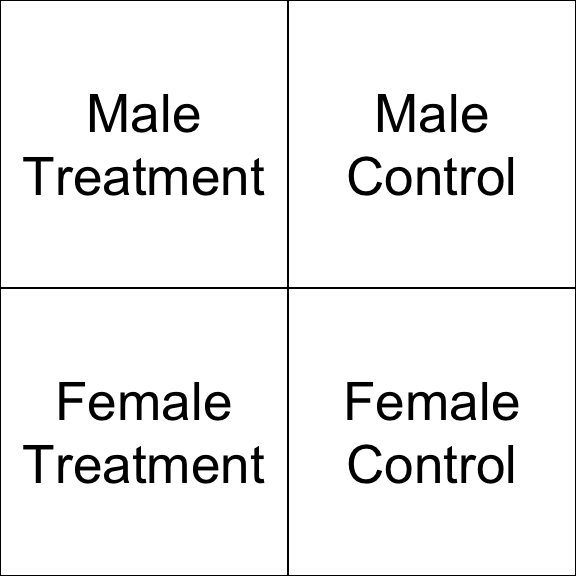
We might be interested in simple groups (treatment cases versus control cases) or complex groups (does the treatment effect women and men differently?).

In previous lectures you have learned to identify a group with a logical statement and analyze that group discretely.

mean( speed[ study.group == "treatment" & gender=="female" ] )
## [1] 608.336

In this lecture you will learn to define a group structure, then analyze all of your data using that structure.

tapply( speed, INDEX = list( study.group, gender ), FUN = mean )
  female male
control 465 358
treatment 608.3 500.6

1.3.2 Main Take-Away

R has been designed to do efficient data analysis by defining a group structure, then quickly applying a function to all unique members.

The base R packages do this with a set of functions in the apply() family. The tapply() function allows you to specify an outcome to analyze and a group, then ask for results from a function.

tapply( X=speed, INDEX=list( study.group, gender ), FUN=mean ) 
  female male
control 465 358
treatment 608.3 500.6

The dplyr package makes this process easier using some simple verbs and the “pipe” operator.

dat  %>%  group_by( study.group, gender )  %>%  summarize( ave.speed = mean(speed) )
study.group gender ave.speed
control male 358
control female 465
treatment male 500.6
treatment female 608.3

1.3.3 Example

Let’s think about a study looking at reading speed. The treatment is a workshop that teaches some speed-reading techniques. In this study we have data on:

  • gender (male, female)
  • race (black, white, asian)
  • blood.type (A, B)
  • age (from 18 to 93)

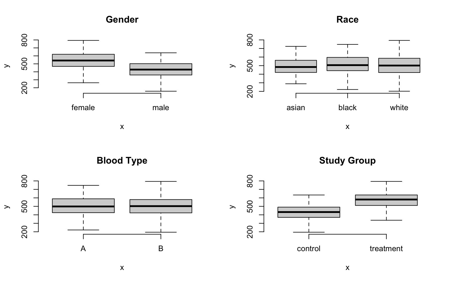
Examining descriptive statistics we can see that reading speed varies by gender and the treatment group, but not by race or blood type:

The question is, how many unique groups can we create with these four factors?

Each individual factor contains a small number of levels (only 2 or 3 in this case), which makes the group structure look deceptively simple at first glance. When we start to examine combinations of factors we see that group structure can get complicated pretty quickly.

If we look at gender alone, we have two levels: male and female. So we have two groups. If we look at our study groups alone we have two groups: treatment and control.

If we look at gender and the study groups together, we now have a 2 x 2 grid, or four unique groups.

If the race factor has three levels, how many unique groups will we have considering the study design, gender, and race together?

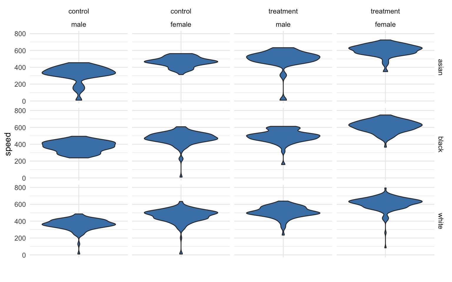
We can calculate the size of the grid by multiplying number of levels for each factor. We see here we have 12 unique groups:

nlevels( gender ) * nlevels( study.group ) * nlevels( race )
## [1] 12

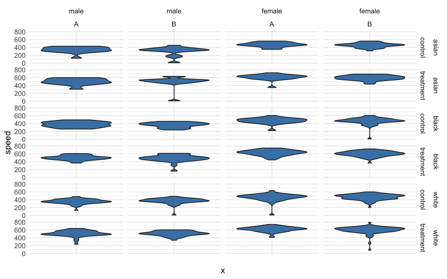
If we add blood type, a factor with two levels (A and B), we now have 24 unique groups:

p + facet_grid( race + study.group ~ gender + blood.type) 

What about age? It is a continuous variable, so it’s a little more tricky.

We can certainly analyze the relationship between age and speed using correlation tools.

plot( age, speed, bty="n", main="Age" )

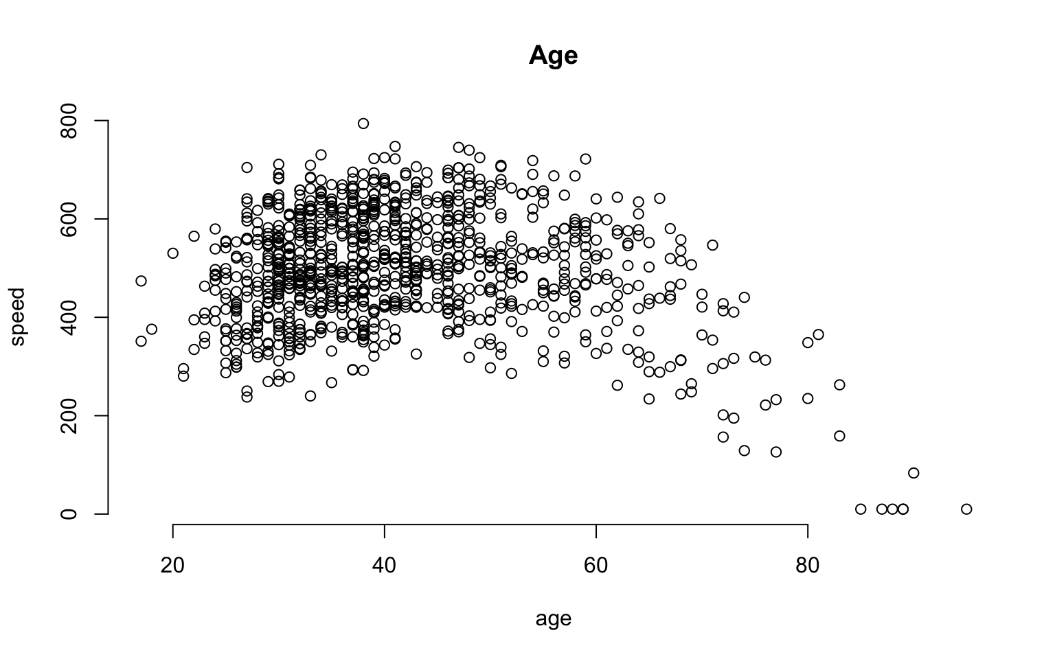
But we can also incorporate this independent variable into a group structure. We can treat each distinct age as a separate group. The ages in this study range from 18 to 93, so we have 65 distinct ages represented.

plot( factor(age), speed, las=2, frame.plot=F, outline=F, main="Age", xaxt="n"  )

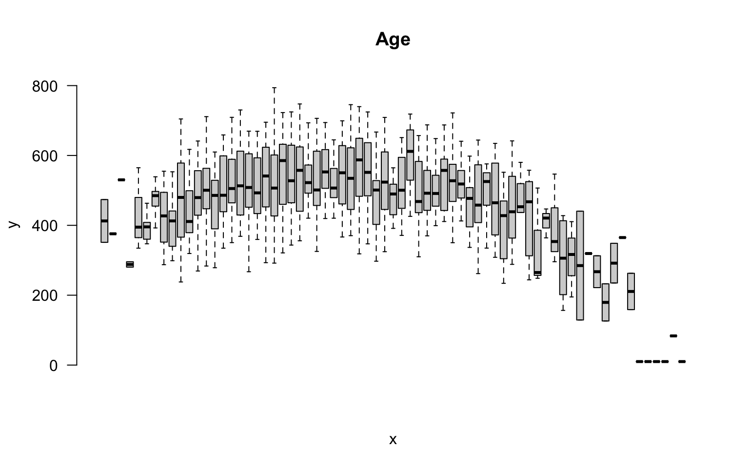
If we think about the overall group structure, then, we have unique groups defined by gender, race, blood type, and study design, and another 65 age groups. So in total we now have 24 x 65 = 1,560 groups! That is getting complicated.

This group design is problematic for two reasons. From a pragmatic standpoint, we can’t report results from 1,500 groups in a table. From a more substantive perspective, although we have 1,500 distinct cells in our grid, many may not include observations that represent the unique combination of all factors. So this group design is not very practical.

A similar problem arises if our data includes time. If our data includes the time of events recorded by hours, days of the week, months, and years, we can have complicated group structures if we try to analyze every unique combination.

We can simplify our analysis by thinking about age ranges instead of ages, or in other words by binning our continuous data. If we split it into five-year ranges, for example, we have gone from 65 distinct ages to 12 distinct age groups.

age.group <- cut( age, 
                  breaks=seq(from=20,to=80,by=5),
                  labels=paste( seq(from=20,to=75,by=5), 
                                "to", seq(from=25,to=80,by=5) ) )

group.structure <- formula( speed ~ age.group )

boxplot( group.structure, las=2, frame.plot=F, outline=F, main="Age Group"  )

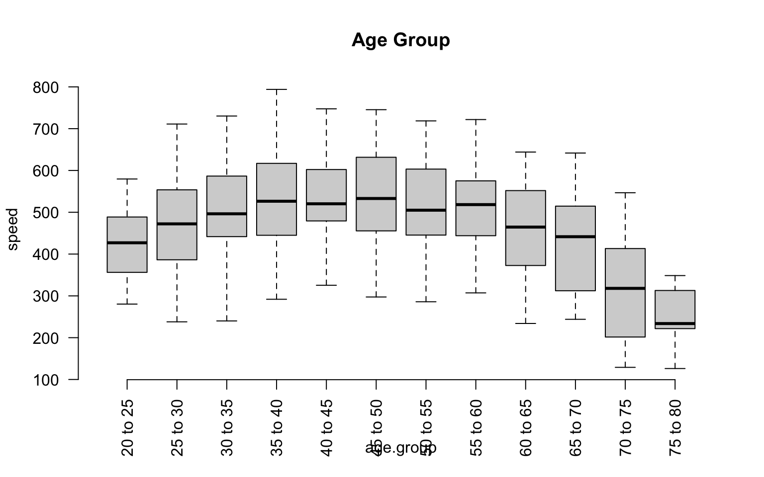
We have now simplified our analysis from 1,560 to 288 possible groups. Combinations of groups will also be easier:

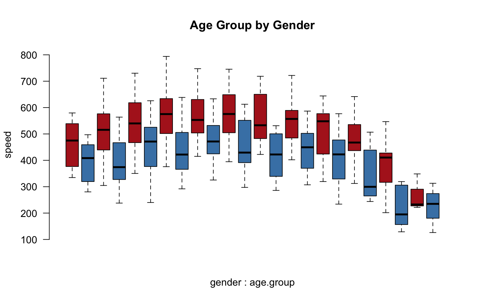
group.structure <- formula( speed ~ gender * age.group )

boxplot( group.structure, 
         las=2, frame.plot=F, outline=F, main="Age Group by Gender",
         col=c("firebrick","steelblue"), xaxt="n" )

1.4 Analysis by Group

Let’s demonstrate some analysis of groups using the Lahman package and some dplyr verbs. Let’s do some analysis of player salaries (Salaries dataset), and start with a simple group structure - teams in the National League and time.

  1. Which team has the highest average player salary?
  2. Which team has the most players paid over $5 million a season?
  3. Which team has raised it’s pay the most over the past decade?

Let’s start by thinking about group structure. We have teams, and we have seasons. Teams is stored as a factor, and seasons as a numeric value, so we can consider group for each by counting levels and unique values:

nlevels( Salaries$teamID )
## [1] 35
length( unique( Salaries$yearID ) )
## [1] 32

So we can potentially calculate 32 x 46 = 1,472 average player salaries.

1.4.1 Highest Average Player Salary

For our first question, we will select only teams from the National League. Let’s use the most recent year of data to calculate average pay.

Salaries %>% filter( lgID == "NL", yearID == 2016 ) %>% 
             group_by( teamID) %>% 
             summarize( Ave_Salary = mean(salary) )
## # A tibble: 15 × 2
##    teamID Ave_Salary
##    <fct>       <dbl>
##  1 ARI      3363041.
##  2 ATL      2362010.
##  3 CHN      5312678.
##  4 CIN      3066899.
##  5 COL      3413487 
##  6 LAN      6322525.
##  7 MIA      2761222.
##  8 MIL      2292508.
##  9 NYN      4958857.
## 10 PHI      2033793.
## 11 PIT      3706387.
## 12 SDN      3756475.
## 13 SFN      6890151.
## 14 SLN      4614629.
## 15 WAS      5448179.

Since the salaries are large, they are a little hard to read. Let’s clean up the table a bit.

Salaries  %>% 
             filter( lgID == "NL", yearID == 2016 ) %>% 
             group_by( teamID ) %>% 
             summarize( Ave_Salary=dollar( mean(salary,na.rm=T) ) ) %>%
             arrange( desc(Ave_Salary) ) %>%
             pander()
teamID Ave_Salary
SFN $6,890,151
LAN $6,322,525
WAS $5,448,179
CHN $5,312,678
NYN $4,958,857
SLN $4,614,629
SDN $3,756,475
PIT $3,706,387
COL $3,413,487
ARI $3,363,041
CIN $3,066,899
MIA $2,761,222
ATL $2,362,010
MIL $2,292,508
PHI $2,033,793

1.4.2 Most Players Paid Over $5 Million

This question requires you to utilize a logical statement in order to translate from the question to code. We need to inspect each salary, determine whether it is over the $5m threshold, then count all of the cases. The operation will look something like this:

sum( Salaries$salary > 5000000 )
## [1] 3175

It gets a little trickier when we want to do the operation simultaneously across groups. Our team group structure is already defined, so let’s define our logical vector and count cases that match:

dat.NL <- filter( Salaries, yearID == 2010 & lgID == "NL" ) %>% droplevels()

gt.5m <- dat.NL$salary > 5000000

table( dat.NL$teamID, gt.5m )
##      gt.5m
##       FALSE TRUE
##   ARI    23    3
##   ATL    21    6
##   CHN    19    8
##   CIN    21    5
##   COL    23    6
##   FLO    23    4
##   HOU    24    4
##   LAN    20    7
##   MIL    25    4
##   NYN    19    9
##   PHI    18   10
##   PIT    27    0
##   SDN    25    1
##   SFN    21    7
##   SLN    19    6
##   WAS    26    4

This solution works, but the table provides too much information. We can use dplyr to simplify and format the table nicely for our report:

Salaries %>% 
   filter( yearID == 2010 & lgID == "NL" ) %>%
   group_by( teamID ) %>% 
   summarise( gt_five_million = sum( salary > 5000000 ) ) %>% 
   arrange( desc(gt_five_million) ) %>%
   pander
teamID gt_five_million
PHI 10
NYN 9
CHN 8
LAN 7
SFN 7
ATL 6
COL 6
SLN 6
CIN 5
FLO 4
HOU 4
MIL 4
WAS 4
ARI 3
SDN 1
PIT 0

1.4.3 Fielding Positions

Which fielding position is the highest paid?

merge( Salaries, Fielding ) %>%
  filter( yearID == 2016 ) %>%
  group_by( POS ) %>%
  summarize( Mean_Salary = dollar( mean(salary) ) ) %>%
  pander
POS Mean_Salary
1B $5,680,014
2B $3,092,188
3B $3,812,355
C $3,167,962
OF $4,317,165
P $4,002,667
SS $2,574,626

1.4.4 Country of Birth

Which country has produced the highest paid baseball players?

merge( Salaries, People ) %>%
  filter( yearID == 2016 ) %>%
  group_by( birthCountry ) %>%
  summarize( Mean_Salary = dollar( mean(salary) ) ) %>% 
  pander
birthCountry Mean_Salary
Aruba $650,000
Australia $523,400
Brazil $1,548,792
CAN $7,854,167
Colombia $3,125,289
Cuba $5,787,593
Curacao $5,724,167
D.R. $5,045,623
Germany $511,500
Japan $8,247,012
Mexico $5,333,671
Netherlands $2,425,000
Nicaragua $2,375,000
P.R. $3,241,378
Panama $2,946,550
Saudi Arabia $522,500
South Korea $5,326,190
Taiwan $6,750,000
USA $4,222,249
V.I. $507,500
Venezuela $4,521,051

1.4.5 Pay Raises

To examine pay raises, we will now use more than one year of data. Since the question asks about pay raises over the past decade, we will filter the last ten years of data.

And since we are looking at patterns over teams and over time, we need to define a group structure with two variables:

Salaries %>% filter( yearID > 2006 & lgID == "NL" ) %>% 
             group_by( teamID, yearID ) %>% 
             summarize( mean= dollar(mean(salary)) ) %>%
             head( 20 ) %>% pander
teamID yearID mean
ARI 2007 $1,859,555
ARI 2008 $2,364,383
ARI 2009 $2,812,141
ARI 2010 $2,335,314
ARI 2011 $1,986,660
ARI 2012 $2,733,512
ARI 2013 $3,004,400
ARI 2014 $3,763,904
ARI 2015 $2,132,207
ARI 2016 $3,363,041
ATL 2007 $3,117,530
ATL 2008 $3,412,189
ATL 2009 $3,335,385
ATL 2010 $3,126,802
ATL 2011 $3,346,257
ATL 2012 $2,856,205
ATL 2013 $3,254,501
ATL 2014 $4,067,042
ATL 2015 $2,990,885
ATL 2016 $2,362,010

This might seem like an odd format. We might expect something that looks more like our grid structure:

dat.NL <- filter( Salaries, yearID > 2010 & lgID == "NL" ) %>% droplevels()

tapply( dat.NL$salary, 
        INDEX=list(dat.NL$teamID, dat.NL$yearID), 
        FUN=mean, na.rm=T ) %>% pander()
  2011 2012 2013 2014 2015 2016
ARI 1986660 2733512 3004400 3763904 2132207 3363041
ATL 3346257 2856205 3254501 4067042 2990885 2362010
CHN 5001893 3392194 3867989 2426759 4138547 5312678
CIN 2531571 2935843 4256178 3864911 4187862 3066899
COL 3390310 2692054 2976363 3180117 3827544 3413487
FLO 2190154 NA NA NA NA NA
HOU 2437724 2332731 NA NA NA NA
LAN 3472967 3171452 6980069 6781706 7441103 6322525
MIA NA 4373259 1400079 1549515 2835688 2761222
MIL 2849911 3755921 3077881 3748778 3477586 2292508
NYN 4401752 3457555 1648278 3168777 3870667 4958857
PHI 5765879 5817965 6533200 5654530 4295885 2033793
PIT 1553345 2248286 2752214 2756357 3065259 3706387
SDN 1479650 1973025 2342339 2703061 4555435 3756475
SFN 4377716 3920689 5006440 5839649 6100056 6890151
SLN 3904947 3939316 3295004 4310464 4586212 4614629
WAS 2201963 2695171 4548131 4399456 5365085 5448179

Later on we will look at the benefits of “tidy data”, but the basic idea is that you can “facet” your analysis easily when your groups are represented as factors instead of arranged as a table. For example, here is a time series graph that is faceted by teams:

Salaries %>% filter( yearID > 2000 & lgID == "AL" ) %>% 
             group_by( teamID, yearID ) %>% 
             summarize( Mean_Player_Salary=mean(salary) ) -> t1

qplot( data=t1, x=yearID, y=Mean_Player_Salary, 
       geom=c("point", "smooth")  ) + 
       facet_wrap( ~ teamID, ncol=5 )

Now you can quickly see that Detroit is the team that has raised salaries most aggressively.

If we need to, we can easily convert a tidy dataset into something that looks like a table using the spread() function:

Salaries %>% filter( yearID > 2006 & lgID == "NL" ) %>% 
             group_by( teamID, yearID ) %>% 
             summarize( mean = dollar(mean(salary)) ) %>%
             spread( key=yearID, value=mean, sep="_" ) %>% 
             select( 1:6 ) %>% na.omit() %>%
             pander
teamID yearID_2007 yearID_2008 yearID_2009 yearID_2010 yearID_2011
ARI $1,859,555 $2,364,383 $2,812,141 $2,335,314 $1,986,660
ATL $3,117,530 $3,412,189 $3,335,385 $3,126,802 $3,346,257
CHN $3,691,494 $4,383,179 $5,392,360 $5,429,963 $5,001,893
CIN $2,210,483 $2,647,061 $3,198,196 $2,760,059 $2,531,571
COL $2,078,500 $2,640,596 $2,785,222 $2,904,379 $3,390,310
FLO $984,097 $660,955 $1,315,500 $2,112,212 $2,190,154
HOU $3,250,333 $3,293,719 $3,814,682 $3,298,411 $2,437,724
LAN $3,739,811 $4,089,260 $4,016,584 $3,531,778 $3,472,967
MIL $2,629,130 $2,790,948 $3,083,942 $2,796,837 $2,849,911
NYN $3,841,055 $4,593,113 $5,334,785 $4,800,819 $4,401,752
PHI $2,980,940 $3,495,710 $4,185,335 $5,068,871 $5,765,879
PIT $1,427,327 $1,872,684 $1,872,808 $1,294,185 $1,553,345
SDN $2,235,022 $2,376,697 $1,604,952 $1,453,819 $1,479,650
SFN $3,469,964 $2,641,190 $2,965,230 $3,522,905 $4,377,716
SLN $3,224,529 $3,018,923 $3,278,830 $3,741,630 $3,904,947
WAS $1,319,554 $1,895,207 $2,140,286 $2,046,667 $2,201,963
Salaries %>% filter( yearID > 2006 & lgID == "NL" ) %>% 
             group_by( teamID, yearID ) %>% 
             summarize( mean = dollar(mean(salary)) ) %>%
             spread( key=teamID, value=mean, sep="_" ) %>% 
             select( 1:6 ) %>% 
             pander
yearID teamID_ARI teamID_ATL teamID_CHN teamID_CIN teamID_COL
2007 $1,859,555 $3,117,530 $3,691,494 $2,210,483 $2,078,500
2008 $2,364,383 $3,412,189 $4,383,179 $2,647,061 $2,640,596
2009 $2,812,141 $3,335,385 $5,392,360 $3,198,196 $2,785,222
2010 $2,335,314 $3,126,802 $5,429,963 $2,760,059 $2,904,379
2011 $1,986,660 $3,346,257 $5,001,893 $2,531,571 $3,390,310
2012 $2,733,512 $2,856,205 $3,392,194 $2,935,843 $2,692,054
2013 $3,004,400 $3,254,501 $3,867,989 $4,256,178 $2,976,363
2014 $3,763,904 $4,067,042 $2,426,759 $3,864,911 $3,180,117
2015 $2,132,207 $2,990,885 $4,138,547 $4,187,862 $3,827,544
2016 $3,363,041 $2,362,010 $5,312,678 $3,066,899 $3,413,487