1 Data Recipes

1.1 Packages Used in This Chapter

library( dplyr )
library( pander )
library( ggvis )

1.2 Key Concepts

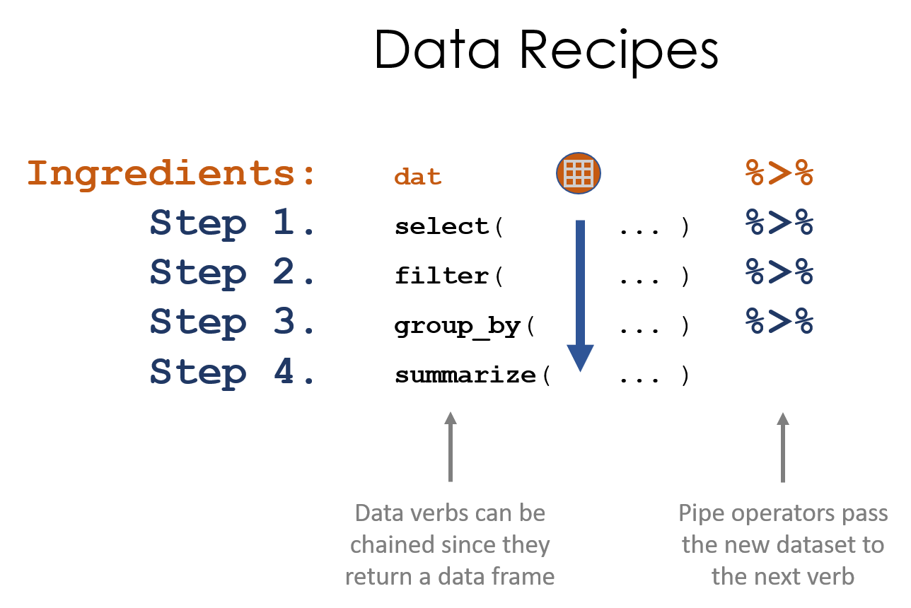
Figure 1.1: Data recipes are written using a series of data steps. We can simplify this process using pipes

Figure 1.2: Recall, data verbs use data frames as the primary input and the output value.

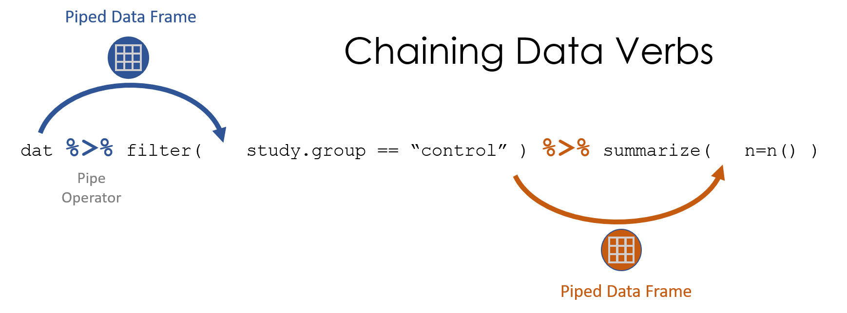
The pipe operator passes a data frame forward through a chain of data verbs. We only reference the dataset name once, and all other times it's implicitly called through piping.

Figure 1.3: The pipe operator passes a data frame forward through a chain of data verbs. We only reference the dataset name once, and all other times it’s implicitly called through piping.

1.3 The Pipe Operator %>%

The idea of functions() was first introduced using a metaphor of a cookie recipe that has ingredients (data and arguments) and requires that each step of the process building on the results of the previous step.

The pipe operator allows us to follow this same model to build “data recipes”, a stylized way of writing a program as a series of data verbs chained together to wrangle and analyze the data. The pipe operator passes the data from one verb to the next without having to name it directly.

Figure 1.4: The pipe operator allows us to pass a transformed dataset forward in the recipe.

1.4 Building Data Recipes

Data recipes are simple scripts that follow a series of steps, just like a recipe.

This chapter demonstrates how data verbs and pipe operators can be used to write recipes to generate interesting insights.

To demonstrate the idea, we will use a dataset of US Baby Names released by the Social Security Administration. This version was downloaded by Ryan Burge and posted on Kaggle. I’ve re-posted it on GitHub so it can be read directly into R easily:

URL <- "https://github.com/DS4PS/Data-Science-Class/blob/master/DATA/BabyNames.rds?raw=true"
names <- readRDS( gzcon( url( URL )))
names %>% head() %>% pander()

Id	Name	Year	Gender	Count
1	Mary	1880	F	7065
2	Anna	1880	F	2604
3	Emma	1880	F	2003
4	Elizabeth	1880	F	1939
5	Minnie	1880	F	1746
6	Margaret	1880	F	1578

Let’s start by building a recipe to identify the top 10 male names for Baby Boomers.

Create a subset of data for men born between 1946 and 1964.
Sort by the annual count of each name in the subset.
Keep only the most popular year for each name.
Identify the top 10 most popular during this period.
Print the results in a nice table that includes name and peak year data.

The recipe will look something like this:

names %>% 
  filter( Gender =="M" & Year >= 1946 & Year <= 1964 ) %>%
  arrange( desc( Count ) ) %>%
  distinct( Name, .keep_all=T ) %>%
  top_n( 10, Count ) %>%
  select( Name, Year, Count ) %>%
  pander()

Name	Year	Count
James	1947	94755
Michael	1957	92709
Robert	1947	91642
John	1947	88318
David	1955	86191
William	1947	66969
Richard	1946	58859
Mark	1960	58735
Thomas	1952	48617
Charles	1947	40773

There are many ways to construct a data recipe. We could have alternatively taken this approach:

Create a subset of data for men born between 1946 and 1964.
Count the total numer of men given each name during the period.
Find the top 10 most popular names.

names %>% 
  filter( Gender =="M" & Year >= 1946 & Year <= 1964 ) %>%
  group_by( Name ) %>%
  dplyr::summarize( total=sum(Count) ) %>%
  dplyr::arrange( desc(total) ) %>%
  slice( 1:10 ) %>%
  pander()

Name	total
James	1570607
Robert	1530527
John	1524619
Michael	1463911
David	1395499
William	1072303
Richard	959321
Thomas	810160
Mark	684159
Charles	657780

We can see that these two approaches to answering our question give us slightly different results, but are pretty close.

Let’s try to identify when specific female names have peaked.

Create a subset of data for women.
Group the data by “Name” so we can analyze each name separately.
Find the year with the highest count for each name.
Store this data as “peak.years”.

Each name will occur once in this dataset in the year that it experienced it’s peak popularity.

peak.years <- 
  names %>%
  filter( Gender == "F" ) %>%
  group_by( Name ) %>%
  top_n( 1, Count ) %>% 
  ungroup() 

peak.years %>% head( 5 ) %>% pander()

Id	Name	Year	Gender	Count
568	Manerva	1880	F	10
720	Neppie	1880	F	7
2621	Zilpah	1881	F	9
4625	Crete	1882	F	8
4750	Alwina	1882	F	6

We can then filter by years to see which names peaked in a given period.

filter( peak.years, Year == 1950 ) %>% 
  arrange( desc( Count ) ) %>%
  slice( 1:5 ) %>%
  pander()

Id	Name	Year	Gender	Count
462006	Constance	1950	F	4442
462008	Glenda	1950	F	4213
462103	Bonita	1950	F	1527
462301	Ilene	1950	F	453
462305	Marta	1950	F	445

# library( ggvis )
names %>%
  filter( Name == "Constance" & Gender =="F" ) %>%
  select (Name, Year, Count) %>%
  ggvis( ~Year, ~Count, stroke = ~Name ) %>%
  layer_lines()

top.five.1920 <- 
  filter( peak.years, Year == 1920 ) %>% 
  top_n( 5, Count ) 

top.five.1920

## # A tibble: 5 × 5
##       Id Name     Year Gender Count
##    <int> <chr>   <int> <chr>  <int>
## 1 169464 Ruth     1920 F      26100
## 2 169465 Mildred  1920 F      18058
## 3 169472 Marie    1920 F      12745
## 4 169477 Lillian  1920 F      10050
## 5 169481 Gladys   1920 F       8819

names %>%
  filter( Name %in% top.five.1920$Name & Gender =="F" ) %>%
  select (Name, Year, Count) %>%
  ggvis( ~Year, ~Count, stroke = ~Name ) %>%
  layer_lines()

top.five.1975 <- 
  filter( peak.years, Year == 1975 ) %>% 
  top_n( 5, Count ) 

names %>%
  filter( Name %in% top.five.1975$Name & Gender =="F" ) %>%
  select (Name, Year, Count) %>%
  ggvis( ~Year, ~Count, stroke = ~Name ) %>%
  layer_lines()

top.five.2000 <- 
  filter( peak.years, Year == 2000 ) %>% 
  top_n( 5, Count ) 

names %>%
  filter( Name %in% top.five.2000$Name & Gender =="F" ) %>%
  select (Name, Year, Count) %>%
  ggvis( ~Year, ~Count, stroke = ~Name ) %>%
  layer_lines()

Ryan Burge posted a fun project on Kaggle about how to find hipster names using this historical data. He defines hipster names as those meeting the following criteria:

They were popular when your grandmother was young.
They were unpopular when your parents were young.
They have recently become popular again.

Let’s stick with women’s names.

df1 <- filter( names, Gender == "F" & Year >= 1915 & Year <= 1935 & Count > 3000 )
df2 <- filter( names, Gender == "F" & Year == 1980 & Count <= 1000 )
df3 <- filter( names, Gender == "F" & Year >= 2010 & Count > 2000)

hipster.names <- 
  names %>%
  filter( Name %in% df1$Name & Name %in% df2$Name & Name %in% df3$Name ) %>%
  group_by( Name ) %>%
  dplyr::summarize( total=sum(Count), peak=max(Count) ) %>%
  arrange( desc( peak ) )

Here are the top 6 female hipster names:

top.hipster.names <- c("Emma","Evelyn","Alice","Grace","Lillian","Charlotte")

names %>%
  filter( Name %in% top.hipster.names & Gender =="F" ) %>%
  select (Name, Year, Count) %>%
  ggvis( ~Year, ~Count, stroke = ~Name ) %>%
  layer_lines()

And the full list:

hipster.names %>% pander()

Name	total	peak
Emma	595546	22701
Evelyn	534502	14279
Grace	469034	12770
Alice	551034	11956
Lillian	421392	10050
Charlotte	312022	10048
Ella	273663	9868
Josephine	297064	8683
Eleanor	268153	8499
Ruby	340143	8407
Hazel	244069	7615
Clara	268980	5779
Eva	252465	4564
Lucy	185064	4257
Stella	155080	4165
Violet	122984	4156
Vivian	198012	4128

1.5 Conclusion

The pipe operator is a little confusing when you first encounter it, but you will find that using data verbs contained in the dplyr package and the pipe operator will speed up your analysis and make your code more readable.

In the next chapter we focus more on the use of groups in data science, and the applications of the group_by() function to make your job easier.