1 DATA VERBS

In this section we are shifting the focus from vector operations to dataset operations.

Some of the most popular packages for building and manipulating datasets come from what is affectionately referred to as the “tidyverse”, a set of packages developed by Hadley Wickam and the R Studio team. They are designed to make basic dataset operations more intuitive and robust.

These packages were created with a common framework for data design called “tidy data”. When datasets are built as or wrangled into the tidy format they are much easier to analyze, and they will play nicely with a large set of packages the follow the same philosophy of data design.

The core R packages contain all of the functions necessary to wrangle datasets, but they are sometimes counter-intuitive or clumbsy in the sense that they might start with a data frame and return a table or a list, making them hard to use in data recipes. All of the “data verbs” that we will cover in this section start with a data frame and return a data frame, making them easier to use as data steps within a larger project.

We will begin with some extremely useful verbs contained within the dplyr package.

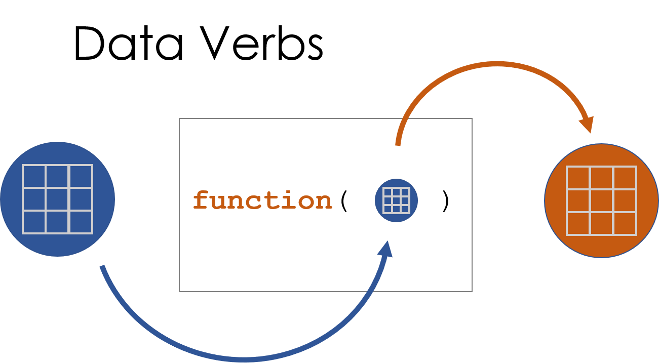
Figure 1.1: A data verb requires a dataset as input, and returns a transformed dataset.

2 The dplyr Package

2.1 Packages Used in This Chapter

library( dplyr )
library( pander )

2.2 Key Concepts

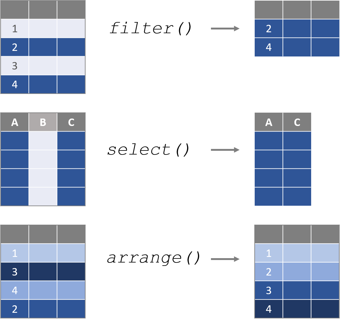
Figure 2.1: Data verbs are functions that require a dataframe as the primary argument, perform some transformation on the data, then return a new dataframe.

For a nice overview of all of the dataset verbs in dplyr check out The dplyr Cheatsheet.

2.3 The dplyr Package

This chapter will demonstrate a few basic dataset functions contained within the dplyr package. There are a few things to note as you get started:

• dplyr functions are all data verbs that accept a dataset as the argument, transform the data, and return a new dataset.
• The first argument is always the dataset name, and variables (columns) can be referenced directly by name without quotation marks.
• dplyr functions will return data as a “tibble” (tbl_df class), which is a regular data frame wrapped in a nice print method that includes metadata in the printout.

For example, here is the regular data frame preview:

##    weight group
## 1    4.17  ctrl
## 2    5.58  ctrl
## 3    5.18  ctrl
## 4    6.11  ctrl
## 5    4.50  ctrl
## 6    4.61  ctrl
## 7    5.17  ctrl
## 8    4.53  ctrl
## 9    5.33  ctrl
## 10   5.14  ctrl

The tibble will print the first few rows and columns of a dataset, and includes dataset dimensions and vector classes:

## # A tibble: 30 × 2
##    weight group
##     <dbl> <fct>
##  1   4.17 ctrl 
##  2   5.58 ctrl 
##  3   5.18 ctrl 
##  4   6.11 ctrl 
##  5   4.5  ctrl 
##  6   4.61 ctrl 
##  7   5.17 ctrl 
##  8   4.53 ctrl 
##  9   5.33 ctrl 
## 10   5.14 ctrl 
## # … with 20 more rows

We will cover the following dplyr functions in this section of the textbook:

DATA VERB	ACTION
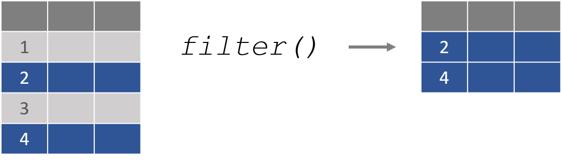
filter()	Select rows
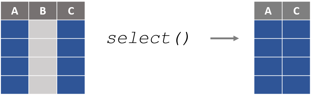
select()	Select columns
arrange()	Sort the dataset by one or more columns
mutate()	Create a new variable by transforming an existing variable or variables
summarize()	Create summary statistics for specified variables
group_by()	Split the dataset (implicitly) into a separate dataset for each group

2.4 Use filter() to Subset Rows

In the last chapter we learned how to use operators to translate from plain English questions to data queries.

As an example, a city manager might want to know the average amount owed on a delinquent property tax.

tax.id	amount.owed
1	$0
2	$5,549
3	$0
4	$1,709
5	$0
6	$634
7	$0
8	$0
9	$0
10	$9,353

We could write the query as follows:

1. Define the group.
2. Select the data that belongs to the group.
3. Analyze the group subset.

these.late <- taxdat$amount.owed > 0                 # 1. Define group
overdue.amounts <- taxdat$amount.owed[ these.late ]  # 2. Select data
overdue.amounts

## [1] 5549 1709  634 9353 1366

mean( overdue.amounts )                              # 3. Analyze data

## [1] 3722.2

The filter() function in the dplyr package is a slightly more elegant verb for selecting the group and subsetting the data by rows.

filter( dataset name , logical expression )

filter( taxdat, amount.owed > 0 )

##   tax.id amount.owed
## 1      2        5549
## 2      4        1709
## 3      6         634
## 4     10        9353
## 5     12        1366

Note that we do not need to reference the dat$ references inside dplyr functions.

2.5 select() Columns

In the core R operators, we select colums from a dataset using the subset function:

data( USArrests ) # historic data on crime rates in the US

	Murder	Assault	UrbanPop	Rape
Alabama	13.2	236	58	21.2
Alaska	10	263	48	44.5
Arizona	8.1	294	80	31
Arkansas	8.8	190	50	19.5
California	9	276	91	40.6
Colorado	7.9	204	78	38.7

USArrests[ , c("Murder","Assault") ]

	Murder	Assault
Alabama	13.2	236
Alaska	10	263
Arizona	8.1	294
Arkansas	8.8	190
California	9	276
Colorado	7.9	204

The select() function converts this operation into a data verb:

select( USArrests, Murder, Assault )

	Murder	Assault
Alabama	13.2	236
Alaska	10	263
Arizona	8.1	294
Arkansas	8.8	190
California	9	276
Colorado	7.9	204

The select() function adds a lot of additional arguments that make it easy to quickly identify and keep only the necessary variables. We can demonstrate a few using the built-in iris dataset in R.

head( iris ) %>% pander()

Sepal.Length	Sepal.Width	Petal.Length	Petal.Width	Species
5.1	3.5	1.4	0.2	setosa
4.9	3	1.4	0.2	setosa
4.7	3.2	1.3	0.2	setosa
4.6	3.1	1.5	0.2	setosa
5	3.6	1.4	0.2	setosa
5.4	3.9	1.7	0.4	setosa

Exclude a column with the negative sign:

select( iris, -Species ) 

Sepal.Length	Sepal.Width	Petal.Length	Petal.Width
5.1	3.5	1.4	0.2
4.9	3	1.4	0.2
4.7	3.2	1.3	0.2
4.6	3.1	1.5	0.2
5	3.6	1.4	0.2
5.4	3.9	1.7	0.4

Select by variable names:

select( iris, ends_with( "Length" ) ) 

Sepal.Length	Petal.Length
5.1	1.4
4.9	1.4
4.7	1.3
4.6	1.5
5	1.4
5.4	1.7

select( iris, starts_with( "Petal" ) ) 

Petal.Length	Petal.Width
1.4	0.2
1.4	0.2
1.3	0.2
1.5	0.2
1.4	0.2
1.7	0.4

select( iris, matches("pal") ) 

Sepal.Length	Sepal.Width
5.1	3.5
4.9	3
4.7	3.2
4.6	3.1
5	3.6
5.4	3.9

Or we can select by a range of variables by placing a colon between the first and last:

select( iris, Sepal.Length:Petal.Width ) 

Petal.Length	Petal.Width	Species
1.4	0.2	setosa
1.4	0.2	setosa
1.3	0.2	setosa
1.5	0.2	setosa
1.4	0.2	setosa
1.7	0.4	setosa

2.6 arrange() Sorts Data

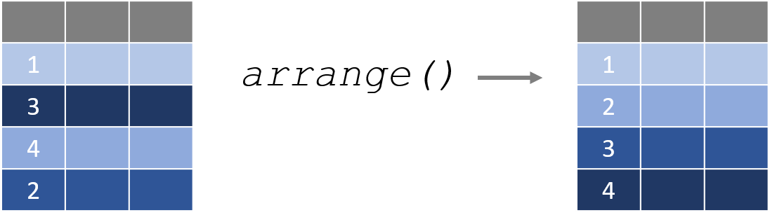
The arrange() function sorts a dataset by one or more columns. By default, it sorts from smallest to largest.

arrange( PlantGrowth, weight ) 

weight	group
3.59	trt1
3.83	trt1
4.17	ctrl
4.17	trt1
4.32	trt1

If we prefer the dataset be sorted from largest to smallest, we can apply the descending function desc() to the sort variable.

arrange( PlantGrowth, desc(weight) ) 

weight	group
6.31	trt2
6.15	trt2
6.11	ctrl
6.03	trt1
5.87	trt1

Or alternatively we can use the shortcut syntax of adding a negative sign in front of the variable:

arrange( PlantGrowth, -weight ) 

We can also sort by multiple columns at once:

arrange( PlantGrowth, group, weight ) 

group	weight
ctrl	5.17
ctrl	5.18
ctrl	5.33
ctrl	5.58
ctrl	6.11
trt1	4.69
trt1	4.81
trt1	4.89
trt1	5.87
trt1	6.03

NOTE, the equivalent core R functions would use subset[] and order() functions together. You might see examples on Stack Overflow written like this:

PlantGrowth[ order(PlantGrowth$weight, decreasing=TRUE) , ]

	weight	group
21	6.31	trt2
28	6.15	trt2
4	6.11	ctrl
17	6.03	trt1
15	5.87	trt1
29	5.8	trt2

As you can see, the dplyr versions are typically more intuitive and concise!

2.7 Variable Transforms with mutate()

One of the most common operations in data analysis is to create a new variable from one or more existing variables, a “variable transformation”. Some examples include:

x_squared <-  x * x

celsius <-  ( fahrenheit - 32 ) * ( 5/9 )

body.mass.index <-  kg / meters^2

per.capita.income <-  income / population

The mutate() function creates a new transformed variable from the formula you specify and adds it to the original dataset.

As an example, perhaps we have data on the number of nonprofits located in each US city. If we look at the raw count of nonprofits, it makes it look as though the large cities have the most vibrant nonprofit sectors:

city	nonprofits
NEW YORK	26503
LOS ANGELES	17417
WASHINGTON	15701
SAN FRANCISCO	12149
BOSTON	10536
CHICAGO	10247
PHILADELPHIA	8538
DALLAS	6008
SEATTLE	5830
ATLANTA	5438

But these numbers may be misleading. Once we account for the population size through a new nonprofit density metric (nonprofits per 1,000 residents), we can see that some smaller cities have higher densities per capita.

dat.npos <- mutate( dat.npos, density = nonprofits / (pop/1000) )

city	density
PORTLAND	2.65
MADISON	2.415
ANCHORAGE	2.156
SANTA BARBARA	1.928
LINCOLN	1.886
WASHINGTON	1.866
ASHEVILLE	1.805
TALLAHASSEE	1.785
BOSTON	1.692
ALBANY	1.685

2.8 rename() Variables

More often than not you will read in a dataset that has strange or meaningless variable names:

x1 <- c("male","male","female","female")
x2 <- c("treatment","control","treatment","control")
dat <- data.frame( x1, x2 )

x1	x2
male	treatment
male	control
female	treatment
female	control

The core R functions make it a little awkward to rename these variables.

names( dat ) <- c("gender","study.group")

gender	study.group
male	treatment
male	control
female	treatment
female	control

The rename() function provides a more intuitive syntax:

rename( dat, gender=x1, study.group=x2 )

2.9 summarize() Variables

The next chapter will cover descriptive statistics in more depth, including some useful packages and functions for generating statistics for a variety of variable types and reporting nice tables.

Most descriptive functions, however, are not data verbs in the sense that they accept a data frame as the input and return a transformed data frame or tibble. The dplyr function summarize() is the primary function that will be used in data recipes (see the next chapter).

Like other data verbs, the first argument will be the input dataset. In this case, there is no pre-determined set of descriptive statistics. The user needs to specify the desired metrics.

group	gender	strength
treatment	male	101
control	male	91
control	male	89
treatment	female	112
control	male	86
control	male	87

summarize( dat, n=n(), min=min(strength), mean=mean(strength), max=max(strength) )

##     n min   mean max
## 1 100  52 100.66 151

Similarly, the native table() function is useful, but returns a table object. The dplyr count() function will function almost identically, but it will return a data frame.

dplyr::count( dat, group, gender )

##       group gender  n
## 1   control female 27
## 2   control   male 26
## 3 treatment female 24
## 4 treatment   male 23

The real power of this function is the ability to use it with the group_by() function to analyze outcomes for many data subsets at once.

grouped.dat <- group_by( dat, group, gender )
dplyr::summarize( grouped.dat, 
                  n=n(), 
                  min=min(strength), 
                  mean=round( mean(strength), 1 ), 
                  max=max(strength) ) 

## # A tibble: 4 × 6
## # Groups:   group [2]
##   group     gender     n   min  mean   max
##   <fct>     <fct>  <int> <dbl> <dbl> <dbl>
## 1 control   female    27    89 116.    151
## 2 control   male      26    52  79.6   125
## 3 treatment female    24    93 115.    144
## 4 treatment male      23    65  91.3   118

We will discuss this functionality in-depth two chapters from now.

Notes for the MS in Program Evaluation and Data Analytics
A program at Arizona State University
Website powered by R Markdown and Jekyll