1 The Grammar of Graphics
1 Key Concepts
In this chapter, we’ll explore the following key concepts:
- Exploratory Data Analysis (EDA)
- Exploratory Data Visualization (EDV)
- Explanatory vs. Explanatory Plots
- The Grammar of Graphics
- Data & Non-Data Ink
- Aesthetic Mappings
- Attributes
- Overplotting
- Faceting
1 New Packages
This chapter uses the following packages:
- ggplot2
- GGally
- scales
- plotly
1 Key Takeaways
Too long; didn’t read? Here’s what you need to know:
- We visualize data to:
- Submit, Publish, Teach (“Explanatory Viz”)
- Explore, Learn, Share (“Exploratory Viz”)
- Exploratory viz is a key part of any data analysis
- “Grammar of Graphics” framework inspired “ggplot2”
- “Layers” are like visual parts of speech
- There are 7 layers - 3 are essential
- Each layer has a family of functions
- Essential layers include:
- Data: Intakes data frame/tibble
- Aesthetic: Maps variables to axes, color, etc.
- Geometry: Specifies the shape of your data
- Nonessential layers include:
- Statistics: Modeling and computation
- Coordinates: Zooming in and modifying scales
- Facets: Small multiples, a.k.a. trellis plots
- Themes: Overall style - grid lines, text, etc.
- Variety of ggplot2 extensions (see resources)
- Use package “plotly” to make ggplot2 interactive
1.1 Why Visualize Data?
We visualize data for two principal reasons. We want to:
- Learn about our data, i.e. exploratory data visualization
- Tell our data’s stories to others, i.e. explanatory data visualization
1.1.1 Explanatory Visualization
Explanatory visualization is polished, publication-quality, and interpretable:
- Meant to be consumed by broad, non-specialist audiences
- Takes significant time and iterations to perfect
- Conveys one or two “big ideas”, each
Just note the length of the code and its result. What idea does this plot convey?
library(ggplot2)

ggplot(read_csv(url), aes(x = val, y = myr)) +
  geom_jitter(alpha = 0.3, color = "tomato") +
  geom_smooth(method = "lm", se = FALSE,
              color = "grey50", lwd = 1, alpha = 0.3) +
  facet_wrap(~ elm) +
  labs(title = "Annual income vs. Holland personality scores",
       x = "Personality Score",
       y = "Income (K)",
       caption = "Sources: US DOL O*NET & BLS") +
  scale_y_continuous(labels = c("0", "50", "100", "150", "$200")) +
  theme_minimal()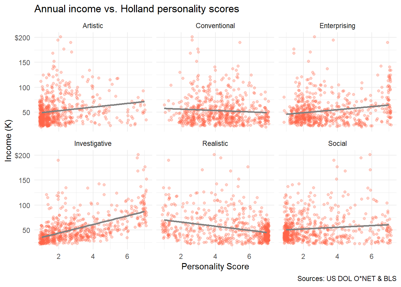
To experiment with Holland codes and predicted income, check it out in Shiny.
1.1.2 Exploratory Visualization
Exploratory visualization is “quick and dirty” and intends to discover.
- Meant to be consumed by yourself, colleagues, or other specialists
- Created quickly, with no polish, refinement, or audience in mind
- Can convey many ideas, or none - that’s why you do it!
This code is manageable! Observe a simple call to ggpairs() and the iris dataset.
library(ggplot2)
library(GGally)

ggpairs(data = iris,
        aes(color = Species))
With just a little code, pairs plots visualize every variable against the other.
Hopefully, you wouldn’t publish this. But we can quickly find patterns in a pairs plot:
- We can see positive correlations between sepal and petals for two species
- We observe that “Setosa” have thinner, longer sepals compared to others
- We also observe that “Versicolor” has the least variation in size
Such visual exploration can help refine hypotheses before analysis begins!
YOUR TURN: EXPLORATORY VIZ WITH PAIRS PLOTS
Load the necessary packages with library().
Then, call ggpairs() on the economics dataset from ggplot2.
1.1.3 Do I have to Visualize?
Exploratory viz is a key component in exploratory data analysis, or EDA.
Failing to visually explore your data can get you in hot water. Let’s try it!
Observe the following data frame containing four data sets.
Variable x1 corresponds to y1, x2 to y2, and so forth:
library(datasets)

anscombe
## x1 x2 x3 x4 y1 y2 y3 y4
## 1 10 10 10 8 8.04 9.14 7.46 6.58
## 2 8 8 8 8 6.95 8.14 6.77 5.76
## 3 13 13 13 8 7.58 8.74 12.74 7.71
## 4 9 9 9 8 8.81 8.77 7.11 8.84
## 5 11 11 11 8 8.33 9.26 7.81 8.47
## 6 14 14 14 8 9.96 8.10 8.84 7.04
## 7 6 6 6 8 7.24 6.13 6.08 5.25
## 8 4 4 4 19 4.26 3.10 5.39 12.50
## 9 12 12 12 8 10.84 9.13 8.15 5.56
## 10 7 7 7 8 4.82 7.26 6.42 7.91
## 11 5 5 5 8 5.68 4.74 5.73 6.89At a glance, they look like the have some similaries!
Check It: Let’s perform a few statistical EDA functions on each subset, 1-4.
What do you notice when we figure out and organize:
- Average of all X and Y values with
mean() - Variance of all X and Y values with
var() - Correlation between X and Y for all sets with
cor() - Linear regression coefficients between X and Y with
lm()
##       x_mean   y_mean x_var    y_var    correl     coeff
## Set 1      9 7.500909    11 4.127269 0.8164205 0.5000909
## Set 2      9 7.500909    11 4.127629 0.8162365 0.5000000
## Set 3      9 7.500000    11 4.122620 0.8162867 0.4997273
## Set 4      9 7.500909    11 4.123249 0.8165214 0.4999091
Heavens to Murgatroyd! These are practically the same sets!
- The mean and variance of X is the exact same across sets
- The mean and variance of Y is almost exactly the same across sets
- The correlation between X & Y is extremely close across sets
- The coefficient of determination is also extremely close
Once visualized, all four linear relationships appear to be exactly the same:
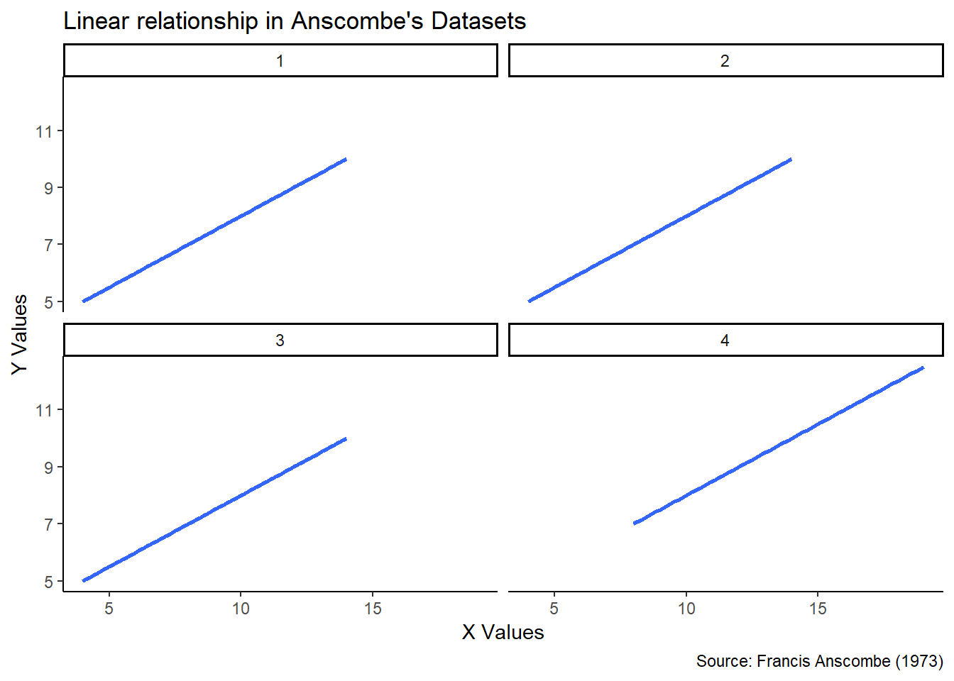
Well, that settles that. Pack it up, folks - the data are the same.
Hold up.
Wait a minute.
Something ain’t right.
Let’s try replotting the actual datasets and not just their linear models.
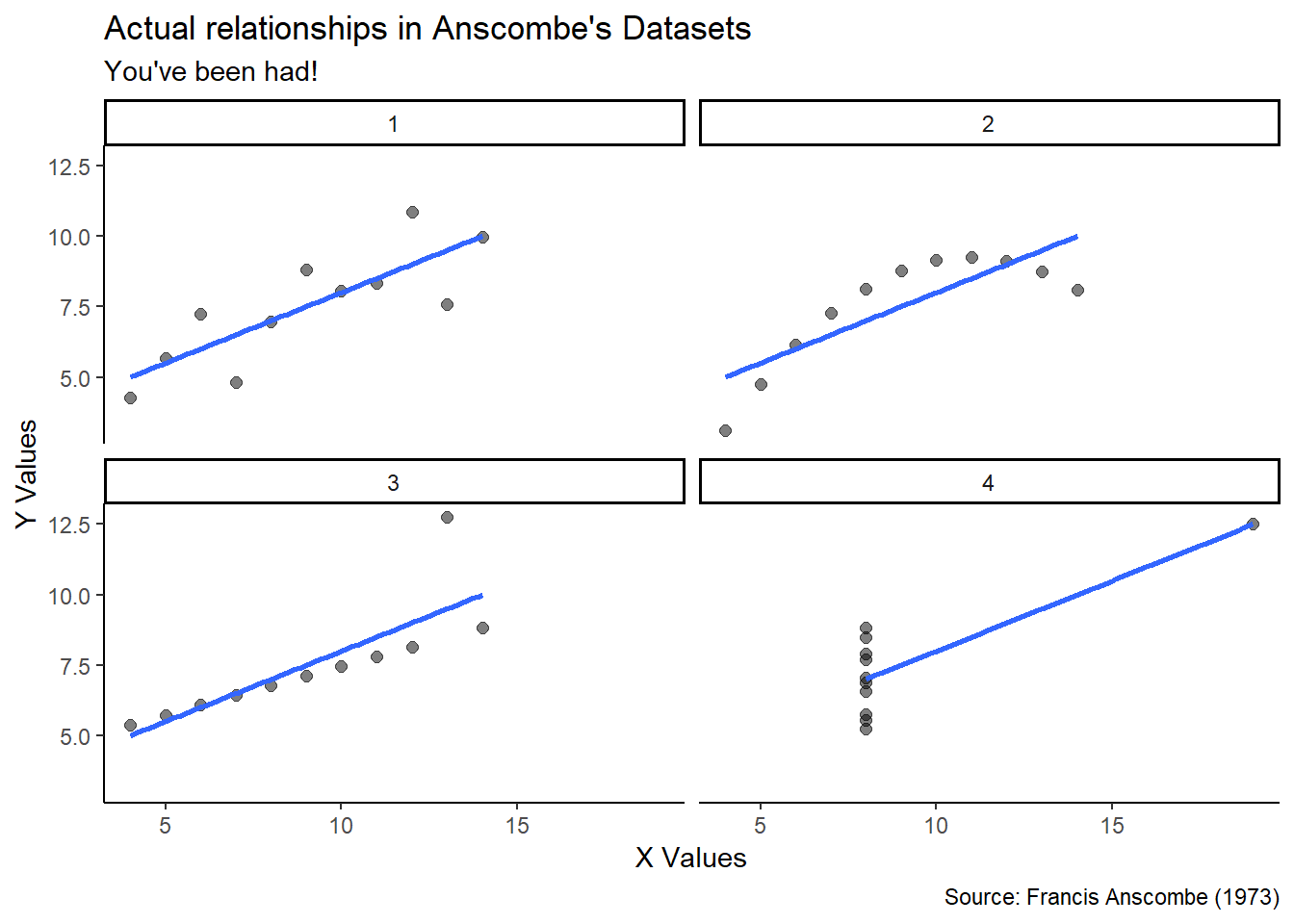
Boom! Not the same datasets at all.
Despite having the same mean, variance, correlations, and coefficients:
- Dataset 1 is a normally distributed linear relationship
- Dataset 2 is a parabolic curve
- Dataset 3 is a perfect linear relationship with a high-leverage outlier
- Dataset 4 shows absolutely no relationship but again has an outlier
Conclusion: Always conduct exploratory visualization as a staple of any analysis.
FUN FACT:
You just got Anscombe’d. Francis John “Frank” Anscombe was an English statistician who helped pioneer the field in the twentieth century. He wrote:
“…a computer should make both calculations and graphs…”
To demonstrate, Anscombe invented these datasets: Anscombe’s Quartet.
1.2 The Grammar of Graphics
We’ve compared human languaes and programming languages in the past.
Let’s take the anology further. Observe the following sentence:
Figure 1.1: The quick brown fox jumps over the lazy dog.
Recall that language consists of nouns, verbs, adjectives, articles, prepositions, etc.
If we change any part of speech, we change the meaning of our sentence. Observe:
The quick brown fox jumps off the lazy dog.
Now the fox has escalated things, opting to use the poor dog as a springboard.
The quick brown fox runs over the lazy dog.
Well this is just getting graphic.
The decrepit brown fox jumps over the lazy dog.
He’s a good dog.
Parts of Speech: Every part of speech (like adjectives, e.g. “quick”, “lazy”) has a function.
Nouns describe things, verbs describe actions, adjectives describe qualities, etc.
Parts of Viz: Like language, there are parts of visualization. Each part has a function.
A chart’s data could be anything, like quarterly revenues or ELA scores
A chart’s geometry could represent the data as bars, points, lines, or shapes
A chart’s theme could use different fonts, gridlines, transparencies, etc.
These are just some parts of viz in a larger framework: The Grammar of Graphics.
1.2.1 A Brief Overview
In 1999, statistician Leland Wilkinson published The Grammar of Graphics.
This framework allows us to dissect and alter plots in the same way we would a sentence.
Let’s begin with parts of viz, or layers.
1.2.2 Layers: Parts of Viz
In the grammar of graphics framework, each visualization is comprised of layers.
- Each layer performs a unique function in a visualization
- Like parts of speech, a layer can perform one function in infinite ways
- For example, the data layer functions to input your data
- A noun can be “fox” or “dog; a dataset can be”DOL" or “TSA”
1.2.3 Essential Layers: Data, Mappings, & Shapes
Like human sentences, every complete visualization has 3 essential layers:
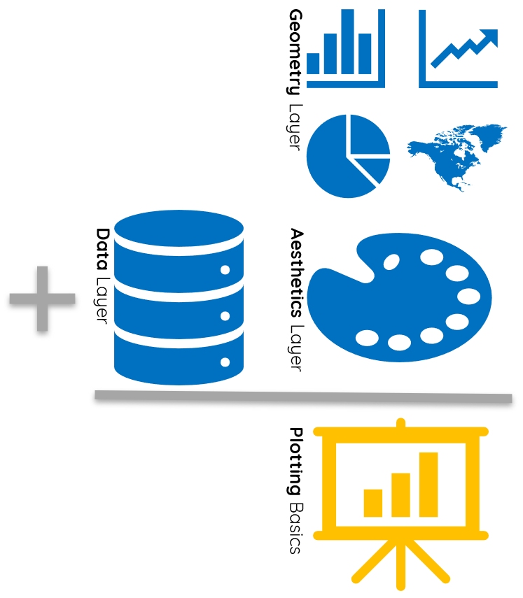
Figure 1.2: The three essential layers for a complete visualization.
1.2.3.1 The Data Layer
The data layer conveys the dataset informing the visualization.
- The data layer inputs a dataset, but doesn’t specify the variables you show
- Visualizations can have more than one data layer, e.g. overlay plots
The data layer in everyday conversation:
"Are you pulling occupations from O*NET or BLS? We only need SOC-level."
Intepretation: Your data layer is comprised of your data source.
Observe the same plot - the only difference is the data layer. What changes?

1.2.3.2 The Aesthetics Layer
The aesthetics layer conveys which variables to visualize.
- Aesthetics refers to the visual ways to represent variables
- Aesthetics include size, shape, color, fill, line type, transparency, etc.
- The most common aesthetic mapping is using x- and y-axes to show quantities
- Aesthetics adjust dynamically with your data - they are not static
The aesthetics layer in everyday conversation:
“Can you color-code the datapoints by gender?”
Intepretation: Aesthetics use visual elements like color to convey more data.
Observe the same plot - the only difference is the aesthetics layer. What changes?
1.2.3.3 The Geometry Layer
The geometry layer conveys the shape your variables use to visualize data.
- Geometries include scatter plots, bar charts, line graphs, etc.
- Some geometries are only compatible with certain variables
- Geometries can also take attributes, like size, shape, color, etc.
- Geometry attributes do not adjust dynamically with data - they are static
The geometry layer in everyday conversation:
“I’m trying to emphasize the increase in elevated blood lead levels over time.”
Intepretation: It sounds like they’d want a line graph or bar chart to show change.
Observe the same plot - the only difference is the geometry layer. What changes?
PRO TIP
It seems like a small distinction, but the difference is critical:
- Both “Attributes” and “Aesthetics” use color, size, line width, fill, etc.
- “Attributes” are static and unchanging
- “Aesthetics” are dynamic and change with your data
All “aesthetics” are specified in the “aesthetics” layer.
All “attributes” are specified in the “geometries” layer.
1.2.4 Remaining Layers
The 4 remaining layers in the grammar of graphics include:
- The coordinates layer modifies plot zoom, truncation, and labeling
- The statistics layer performs statistical transformations like lines of best fit
- The facets layer creates multiple comparison plots, a.k.a. small multiples
- The themes layer modifies font, gridlines, and other “non-data ink” polish
We’ll explore some key functions from these layers in the following sections.
1.3 Download the Practice Data
Our practice data are public consruction project worker records in Syracuse, NY.
They were collected for a racial equity impact statement on hiring disparities.
Download: You can download the practice data here.
To Follow Along: Run this code in your R console:
library(readr)

url <- paste0("https://raw.githubusercontent.com/DS4PS/",
              "dp4ss-textbook/master/tables/hancock.csv")

hancock <- read_csv(url)

rm(url)
Figure 1.3: The impact statement uses ggplot2 for the majority if its viz (p. 95).
1.4 Package “ggplot2”
Package “ggplot2” is a popular, powerful package for data visualization in R.
- Authored by Hadley Wickham; maintained by RStudio
- An implementation of the “Grammar of Graphics” framework (hence “gg”)
- Has a series of function families, each corresponding to a different layer
Expressions in “ggplot2” use a particular syntax. Note that + connects the layers.
Let’s look at a “complete” graph:
library(ggplot2)

ggplot(data = hancock) +      # Data layer
  aes(x = net) +              # Aesthetics layer
  geom_histogram()            # Geometry layer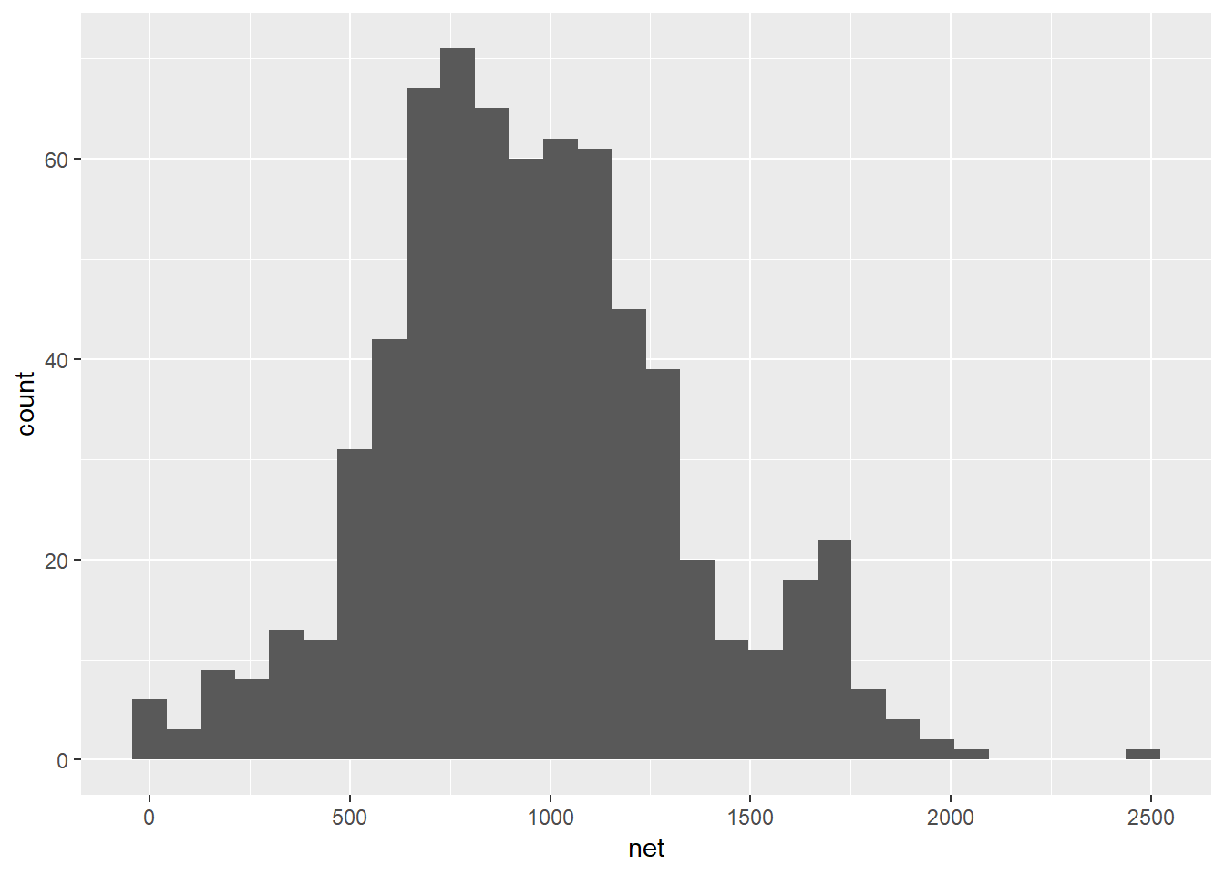
Note that the preferred “ggplot2” format is as follows (both do the same thing):
ggplot(data = hancock,
       aes(x = net)) +        # "aes()" is nested in "ggplot()"
  geom_histogram()
Let’s break it down. Here are the three layers of a “ggplot2” graphic and how they work:
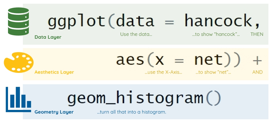
Figure 1.4: Breaking down a “complete” graphic.
YOUR TURN: A BASIC GGPLOT
- Load the necessary packages with
library() - Call
ggplot()on theeconomicsdataset from ggplot2 - In
aes(), map x = todateand y = tounemploy - Call
geom_line()
A call to theme_classic() has been added for panache.
Adding Aesthetics: Let’s plot the same data, except with:
aes()argument x = mapped tonetaes()argument y = mapped togrossgeom_histogram()changed togeom_point()
ggplot(data = hancock,
       aes(x = net,
           y = gross)) +    # Now mapping "gross" to y-axis
  geom_point()              # Changed from geom_histogram()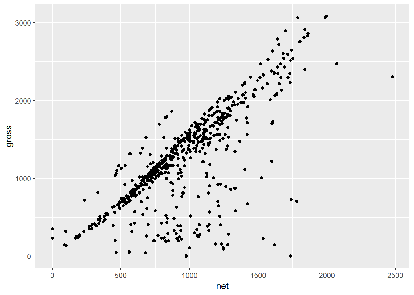
Modifying Attributes: We can change attributes (non-data ink) in the geom_*() call.
- Modify transparency with argument alpha =
- Modify color and fill with color = and fill =, respectively
ggplot(data = hancock,
       aes(x = net,
           y = gross)) +
  geom_point(alpha = 0.35,        # Modify transparency between 0 & 1
             color = "tomato")    # Modify color; some colors are known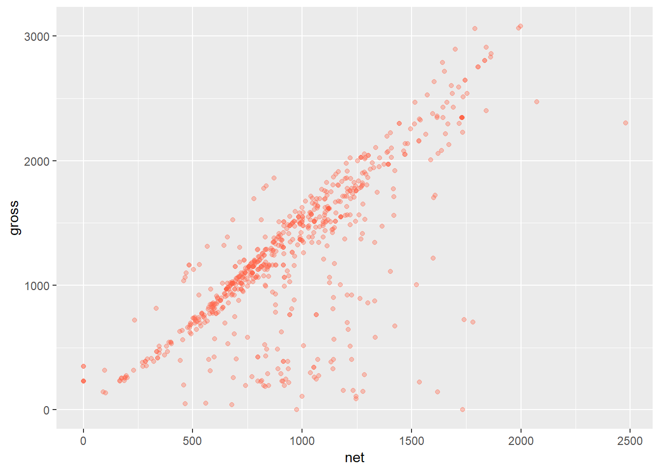
Modify Labels: We can add function labs() with + to modify labels and titles:
ggplot(data = hancock,
       aes(x = net,
           y = gross)) +
  geom_point(alpha = 0.35,
             color = "tomato") +
  labs(title = "Weekly gross v. net incomes in public construction",
       subtitle = "Hancock Airport, 2018",
       x = "Net Earnings",
       y = "Gross Earnings",
       caption = "Source: Syracuse Regional Airport Authority")
Premade Themes: Add premade themes with + and theme_ functions:
ggplot(data = hancock,
       aes(x = net,
           y = gross)) +
  geom_point(alpha = 0.35,
             color = "tomato") +
  labs(title = "Weekly gross v. net by public construction workers",
       subtitle = "Hancock Airport, 2018",
       x = "Net Earnings",
       y = "Gross Earnings",
       caption = "Source: Syracuse Regional Airport Authority") +
  theme_minimal()                                                   # New theme
Conclusions: In package “ggplot2”, we build on these three essential layers.
- The data layer, the aesthetics layer, and the geometry layer
- Call data, aesthetics, and geometry in
ggplot(),aes(), andgeom*()functions - Once you’ve build an initial plot, you can add new layers to enhance it, like themes
- Each addition makes plots more decodable and better emphasizes big ideas
YOUR TURN: AESTHETICS & ATTRIBUTES
A basic ggplot has been prepared for you.
Load the necessary packages with library().
Modify geom_point() with the following:
- Set size to 2.75 (size =)
- Set transparency to 0.15 (alpha =)
- Set color to “darkslateblue” (color = )
A theme_minimal() is provided for panache.
1.5 Notable Layer Functions
Each layer in “ggplot2” has an astounding number of functions. Let’s check some out.
1.5.1 The Aesthetics Layer
We’ve seen the principal function of the aesthetics layer, aes().
Most importantly, you should some arguments to which you can map variables:
- x = maps to the x-axis
- y = maps to the y-axis
- z = maps to the z-axis (3-dimensional, typically)
- color = maps to colors of points and lines
- fill = maps to colors of shapes, e.g. bars
- size = maps to the size of points
- labels = maps to the labels of points, lines, and shapes
- width = maps to the width of lines
- type = maps to the line type
Read more about aesthetics in the “ggplot2” vignette.
Take the following scatter plot of U.S. unemployed against total population since 1970:
library(ggplot2)

ggplot(data = economics,
       aes(x = unemploy,
           y = pop)) +
  geom_point() +
  theme_minimal()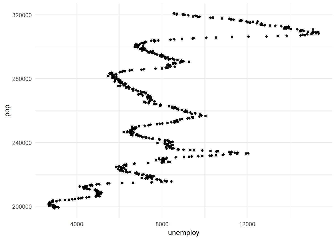
We can convey additional information by mapping aesthetics to other variables.
The following maps point size to psavert, or the personal savings rate.
library(ggplot2)

ggplot(data = economics,
       aes(x = unemploy,
           y = pop,
           size = psavert)) +     # Map personal savings rate to size
  geom_point(alpha = 0.2) +       # Set transparency to 20%
  theme_minimal()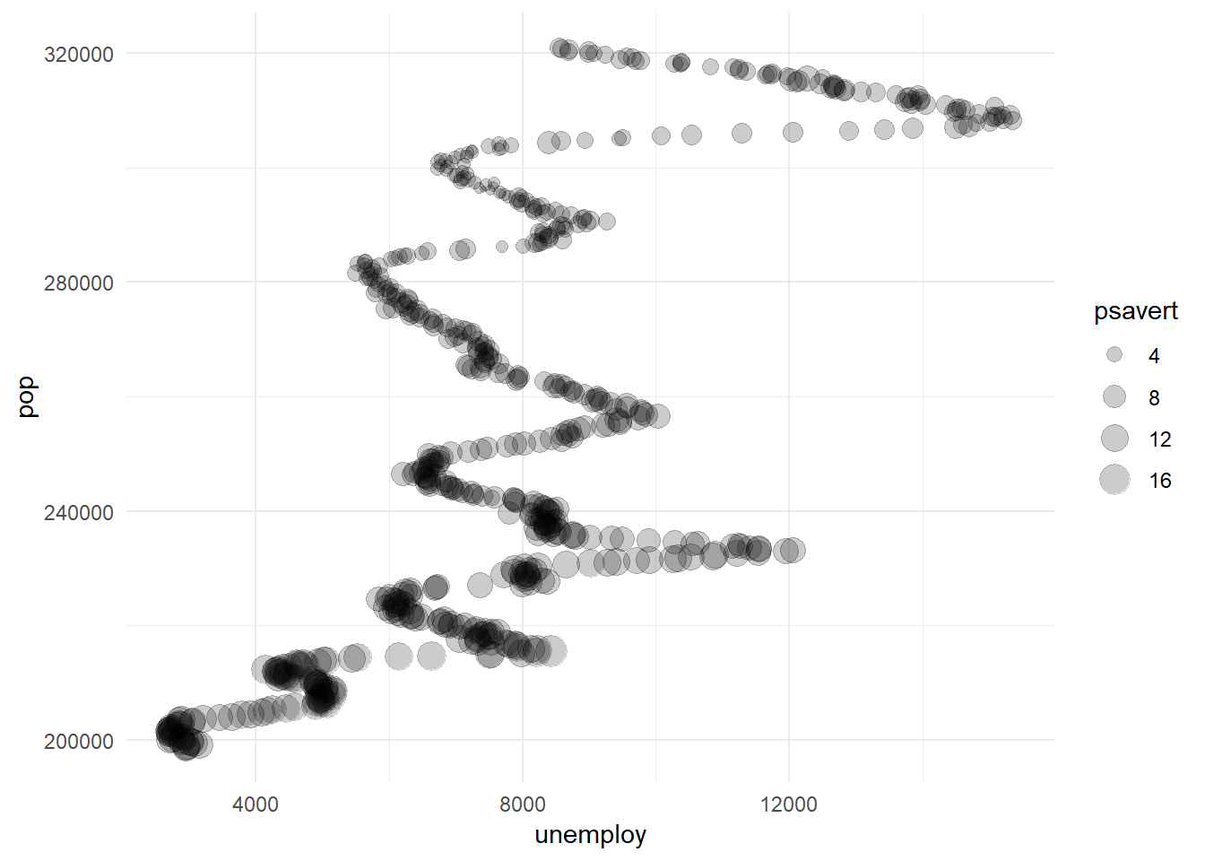
We can see that regardless of unemployment, savings dwindle as populations grow.
(Population, by the way, is practically interchangeable with date).
CAUTION: OVERPLOTTING & OVERMAPPING
It’s tempting to map many variables to different aesthetics, so be careful to not:
- “Overplot”, or obfuscate clarity with too many mappings
- “Overmapping”, or mapping a variable to two or more aesthetics
For example, don’t map “population”, e.g. to both color and the y-axis.
- As datapoints move upward on the y-axis, the color changes
- It may make your plot pretty, but it makes it harder to decode
- What’s more, color is redundant and pointless - axes are more decodable
- In effect, this is known in data visualization as “belt-and-suspenders design”
Belts or suspenders… you don’t need both!
1.5.2 The Geometry Layer
Each shape your data takes in the geometry layer has an associated function.
- View all geometries on the “ggplot2” reference page
- Notably, every geometry function begins with
geom_ - Some statistical functions have equivalents that begin with
stat_ - You can combine more than one geom function in a singple visual
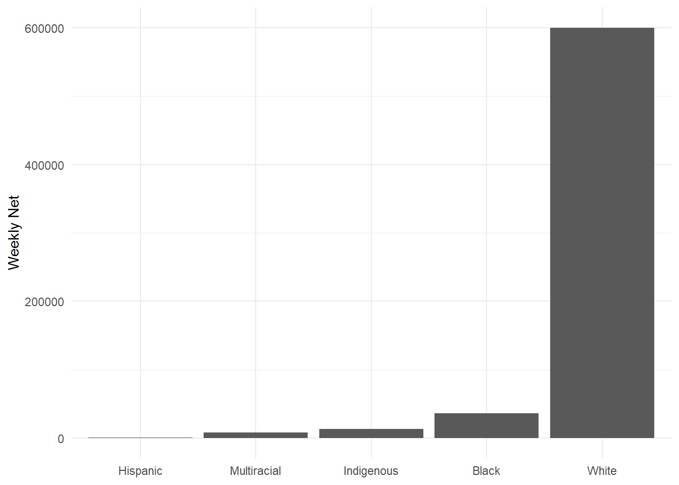
Rectangular Geoms: When using geoms with rectangular shapes, set stat = to “identity”.
options(scipen = 999)                       # Disable scientific notation

ggplot(data = hancock,
       aes(x = reorder(ethnicity, -net),    # Reorder ethnicities by "net"
           y = net)) +
  geom_bar(stat = "identity") +             # Specify stat = "identity"
  labs(x = NULL,
       y = "Weekly Net") +
  theme_minimal()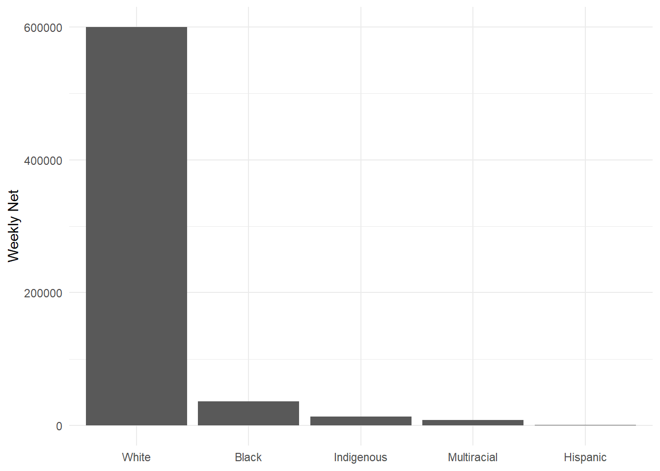
Use Fill to Modify Geoms: Map aes() argument fill = to a categorical variable:
ggplot(data = hancock,
       aes(x = reorder(ethnicity, -net),
           y = net,
           fill = reorder(class, -net))) +  # Add fill = and reorder() on "net"
  geom_bar(stat = "identity") +
  labs(x = NULL,
       y = "Weekly Net",
       fill = "Class") +                    # Use labs() and fill= to title legend
  theme_minimal()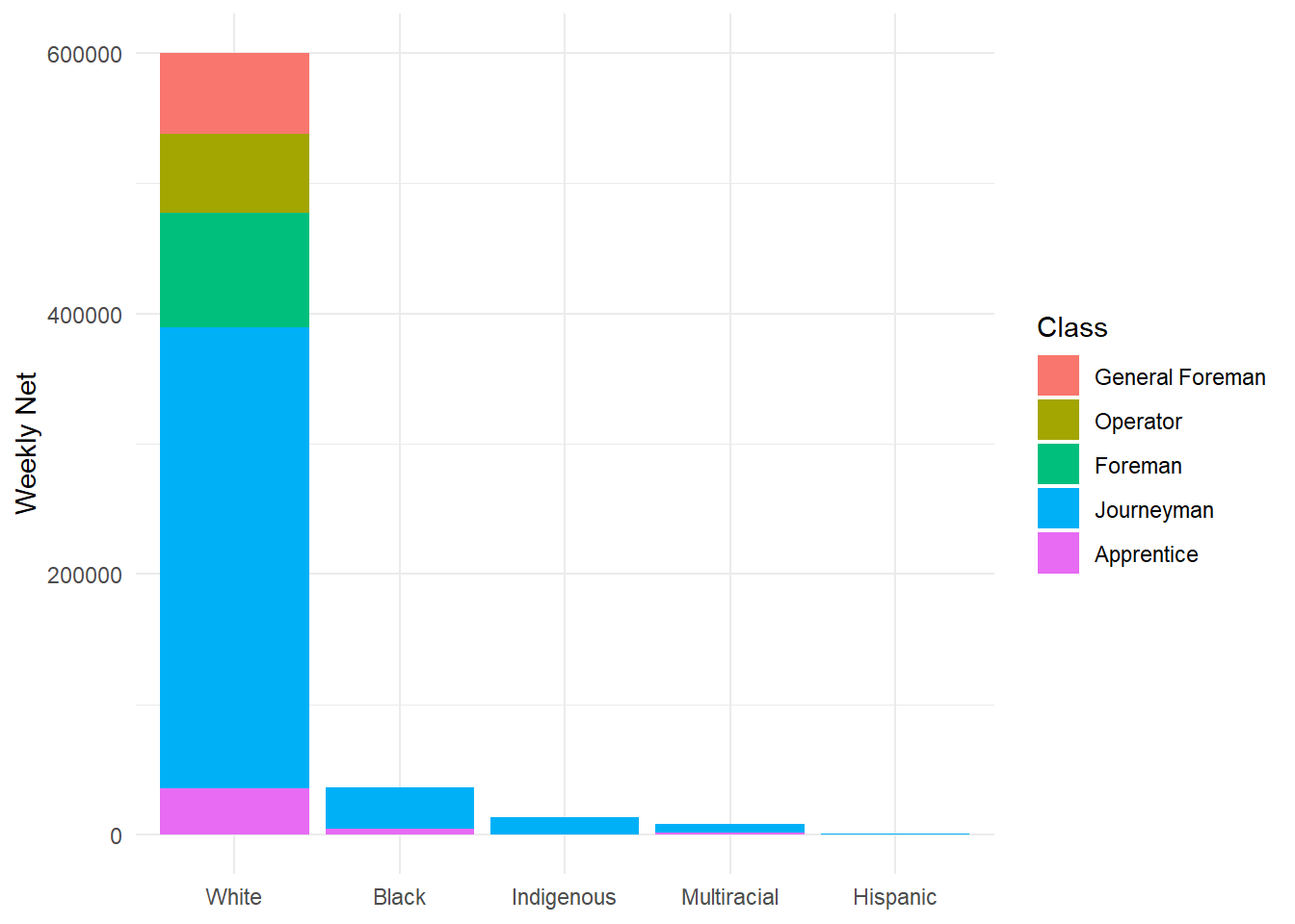
Fill to 100%: With a fill = asthetic, set position = to “fill”:
ggplot(data = hancock,
       aes(x = reorder(ethnicity, -net),
           y = net,
           fill = reorder(class, -net))) +
  geom_bar(stat = "identity",
           position = "fill") +             # Set position = to "fill"
  labs(x = NULL,
       y = "Weekly Net",
       fill = "Class") +
  theme_minimal()
New Geoms with New Positions: With a fill = asthetic, set position = to “dodge”:
ggplot(data = hancock,
       aes(x = reorder(ethnicity, -net),
           y = net,
           fill = reorder(class, -net))) +
  geom_bar(stat = "identity",
           position = "dodge") +            # Set position = to "dodge"
  labs(x = NULL,
       y = "Weekly Net",
       fill = "Class") +
  theme_minimal()
Overlapping Barplots: Set position = to position_dodge() and set width =:
ggplot(data = hancock,
       aes(x = reorder(ethnicity, -net),
           y = net,
           fill = reorder(class, -net))) +
  geom_bar(stat = "identity",
           position = position_dodge(width = 0.5)) +            # Control the dodge!
  labs(x = NULL,
       y = "Weekly Net",
       fill = "Class") +
  theme_minimal()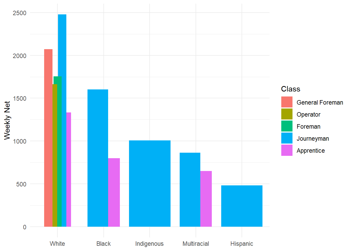
FUN FACT
Many ggplot2 color functions contain brewer in the name. That’s because, by default, ggplot2 uses color palettes based on the research of Dr. Cynthia Brewer.
Dr. Brewer’s premade palettes, all recognized in ggplot2, are available in Color Brewer 2.
Overlap & Transparency: When multiple points overlap, use transparency (alpha =).
ggplot(data = hancock,
       aes(x = reorder(ethnicity, -net),
           y = net)) +
  geom_point(alpha = 0.10) +          # Set transparency to 10%
  labs(x = NULL,
       y = "Weekly Net") +
  theme_minimal()
Overlapping & Jittering: In combination with transparency, you can “jitter” your points.
- “Jittering” adds random horizontal and vertical noise to break up points
- In function
geom_point(), set position = to “jitter” - Arguments height = and width = controls jitter
- Alternatively, use function
geom_jitter()
ggplot(data = hancock,
       aes(x = reorder(ethnicity, -net),
           y = net)) +
  geom_jitter(alpha = 0.15,           # Change geom to geom_jitter()
              width = 0.25) +         # Set "jitter" width to 0.25
  labs(x = NULL,
       y = "Weekly Net") +
  theme_minimal()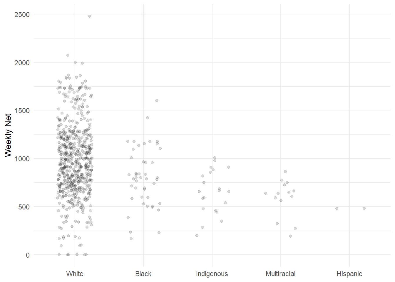
YOUR TURN: JITTER & TRANSPARENCY
Load the necessary packages with library().
Then, call ggplot() on the midwest dataset from ggplot2.
- Change
geom_point()togeom_jitter() - In
geom_jitter(), set argument alpha = 0.25 - Also in the geom, set argument width = 0.15
1.5.3 The Statistics Layer
The statistics layer is where data undergo statistical transformations under the hood.
- All stat layer functions begin with
stat_ - Many geometries already use stats, like
geom_smooth() - Argument method = can use different models with “lm”, “glm”, “rlm”, etc.
- Stat functions typically not called directly, but run within geom functions
Smoothers: Function stat_smooth() adds a LOESS line and standard error area.
ggplot(hancock,
       aes(x = net,
           y = gross)) +
  geom_point() +
  stat_smooth() +                 # Function stat-smooth(), same as geom_smooth()
  theme_minimal()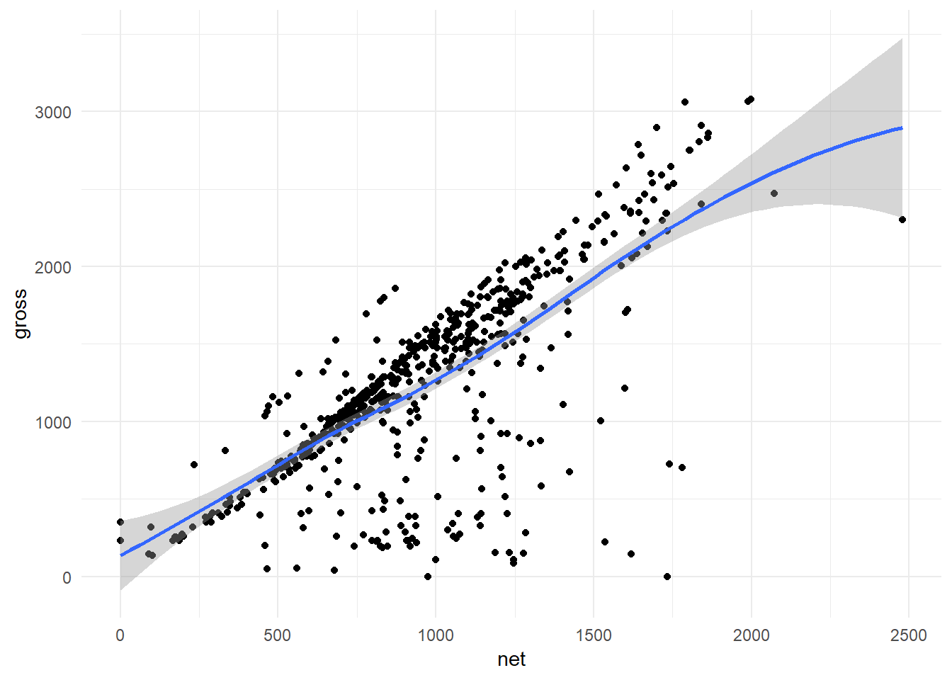
Remove Standard Error: Set argument se = to FALSE to disable standard error.
ggplot(hancock,
       aes(x = net,
           y = gross)) +
  geom_point() +
  stat_smooth(se = FALSE) +       # Argument se = controls standard error
  theme_minimal()
Chane Modeling Method: Set argument method = to “lm” for linear models, etc.
ggplot(hancock,
       aes(x = net,
           y = gross)) +
  geom_point() +
  stat_smooth(se = FALSE,
              method = "lm") +    # Argument method = changes your model
  theme_minimal()
1.5.4 The Coordinates Layer: Planes
The coordinates layer ultimately controls the limits and labels of your axes.
- All coordinates functions begin with
coord_ - Most common is
coord_cartesian(), which modifies a plot’s Cartesian plane
Flipping Coordinates! No, we’re not cursing out coordinates.
However, you can reverse the x- and y-axes by using function coord_flip():
options(scipen = 999)                 # Disable scientific notation

ggplot(data = hancock,
       aes(x = reorder(ethnicity, net),
           y = net)) +
  geom_bar(stat = "identity") +
  labs(title = "Flipped!",
       x = NULL,
       y = "Weekly Net") +
  theme_minimal() +
  coord_flip()                        # coord_flip() !
Zooming or Filtering: Modifying coordinates typically goes one of two ways:
- Zoom in on some specified coordinates
- Zoom in and filter out data that are no longer visible
Zoom with coord_cartesian().
Filter with lims().
The Whole Plot (Before): Observe the entirety of the plot without zooming in:
ggplot(hancock,
       aes(x = net,
           y = gross)) +
  geom_point() +
  geom_smooth() +
  theme_minimal()
Zoomed In: We can zoom, without affecting our data, with coordcartesion().
Note the direction and standard error of the LOESS line from geom_smooth().
ggplot(hancock,
       aes(x = net,
           y = gross)) +
  geom_point() +
  geom_smooth() +
  theme_minimal() +
  coord_cartesian(xlim = c(0, 1250),
                  ylim = c(0, 2000))    # Zoom in and keep your data!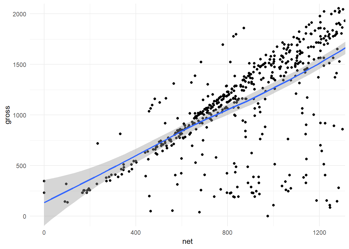
Filtered: We can use lims() to zoom in and filter data no longer plotted.
Now note how the LOESS line and standard error have changed per this “new” dataset.
ggplot(hancock,
       aes(x = net,
           y = gross)) +
  geom_point() +
  geom_smooth() +
  theme_minimal() +
  lims(x = c(0, 1250),
       y = c(0, 2000))                  # Zoom in and filter your data!
QUESTION
Why do the LOESS curves and standard errors change between plots?
1.5.5 The Coordinates Layer: Scales
Scales in “ggplot2” affect your axis gridlines, ticks, breaks, and labels.
- Scale functions begin with
scale_ - Specify which axis with
scale_x_orscale_y_ - Also specify
discrete,continuous, or another variable type - Example: A discrete (categorical) variable on the y-axis is
scale_y_discrete()
Axis Titles: Change (or remove) axis titles with argument name =:
ggplot(hancock,
       aes(x = net,
           y = gross)) +
  geom_point(alpha = 0.05) +
  geom_smooth(color = "grey80", alpha = 0.1) +
  theme_minimal() +
  scale_x_continuous(name = "Weekly Net") +     # Axis? Continuous or discrete?
  scale_y_continuous(name = "Weekly Gross")     # Argument name = for axis titles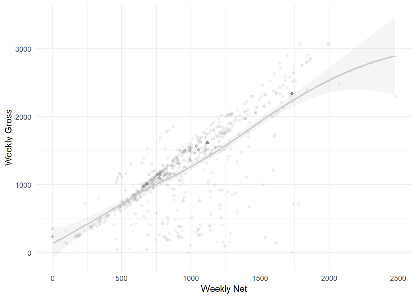
Breaks: Specify axes’ major label and tick marks with argument breaks = and c():
ggplot(hancock,
       aes(x = net,
           y = gross)) +
  geom_point(alpha = 0.05) +
  geom_smooth(color = "grey80", alpha = 0.1) +
  theme_minimal() +
  scale_x_continuous(name = "Weekly Net",
                     breaks = c(0, 1250, 2500)) +
  scale_y_continuous(name = "Weekly Gross",
                     breaks = c(0, 1500, 3000))           # Even breaks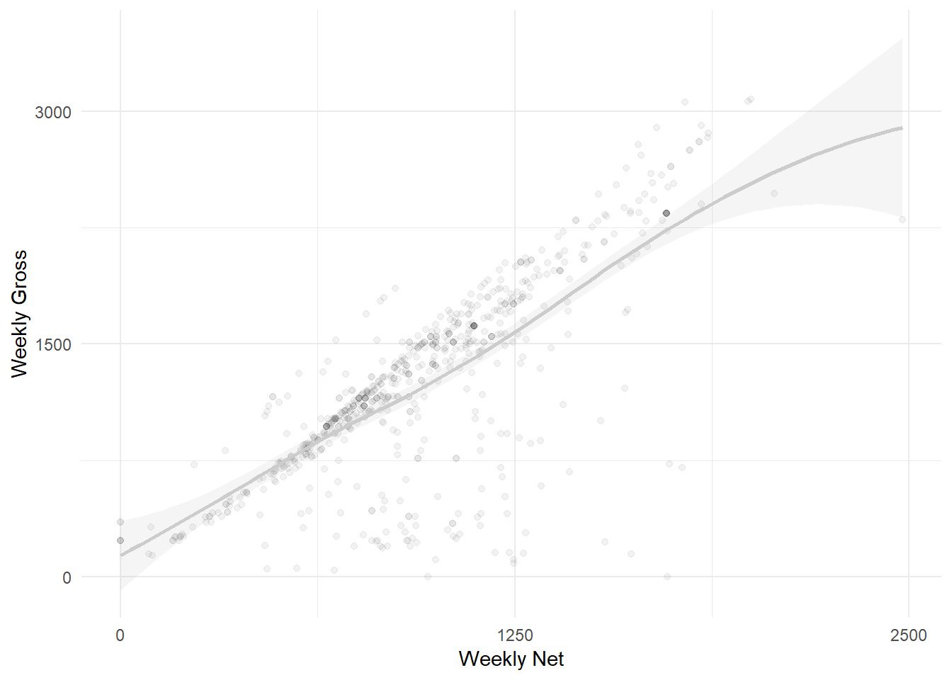
Labels: Customize individual labels with argument labels = (ojo - can get lengthy):
ggplot(hancock,
       aes(x = net,
           y = gross)) +
  geom_point(alpha = 0.05) +
  geom_smooth(color = "grey80", alpha = 0.1) +
  theme_minimal() +
  scale_x_continuous(name = "Net",
                     breaks = c(0, 1250, 2500),
                     labels = c("$ 0", "1.25", "2.5 K")) +
  scale_y_continuous(name = "Gross",
                     breaks = c(0, 1500, 3000),
                     labels = c("$ 0", "1.5", "3 K"))     # Labels in quotes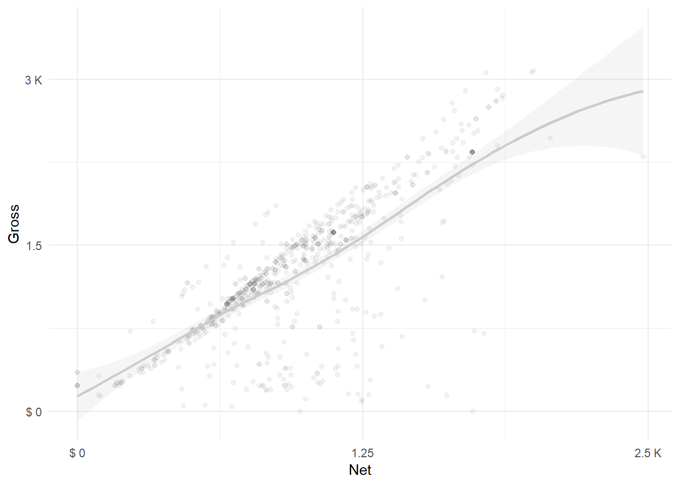
Pretty Breaks: Package “scales” allows us to more easily format scale_*() functions.
- Format breaks automatically (pretty-like)
- Label dollar amounts and percentages with ease
Pretty Names: With “scales”, argument name = accepts new standards:
library(scales)

ggplot(hancock,
       aes(x = net,
           y = gross)) +
  geom_point(alpha = 0.05) +
  geom_smooth(color = "grey80", alpha = 0.1) +
  theme_minimal() +
  scale_x_continuous(name = "Net",
                     breaks = c(0, 1250, 2500),
                     labels = dollar) +                   # Auto-labeling: Good
  scale_y_continuous(name = "Gross",
                     breaks = c(0, 1500, 3000),
                     labels = dollar)                     # Less flexibility: Bad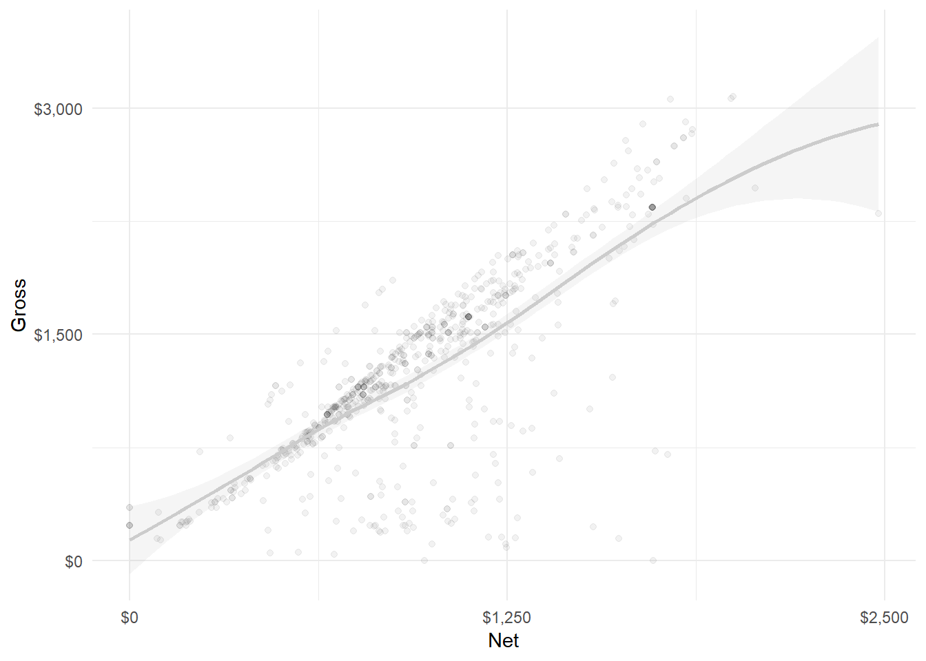
Pretty Breaks: With “scales”, argument breaks = accepts pretty_breaks():
library(scales)

ggplot(hancock,
       aes(x = net,
           y = gross)) +
  geom_point(alpha = 0.05) +
  geom_smooth(color = "grey80", alpha = 0.1) +
  theme_minimal() +
  scale_x_continuous(name = "Net",
                     breaks = pretty_breaks(5),
                     labels = dollar) +                   # pretty_breaks() !
  scale_y_continuous(name = "Gross",
                     breaks = pretty_breaks(12),
                     labels = dollar)                     # Pretty sick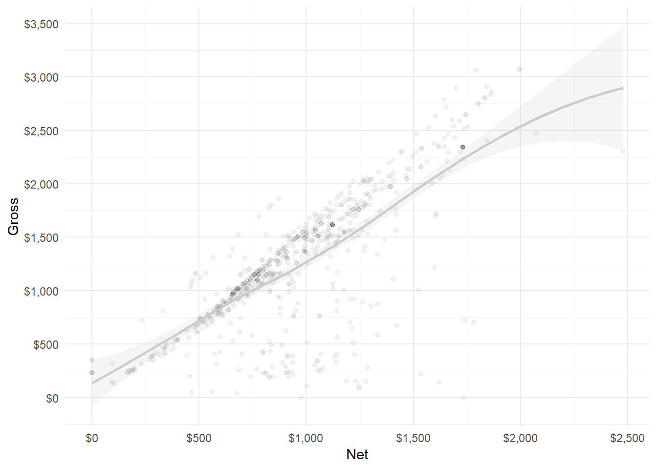
PRO TIP: PACKAGE “SCALES” APPLICATIONS
The “scales” package has a host of amazing formatting functions. Commonly:
dollar()anddollar_format()for currencypercent()andpercent format()for percentsnumber()andnumber_format()for numbers
These and other functions are incredibly useful, especially for cleaning.
YOUR TURN: STATS, COORDINATES, AND SCALES
Load the necessary packages with library().
- In
geom_point(), set “alpha = 0.3” - Add
geom_smooth()with+ - Add
lims()with:- x =
c(0, 10000) - y =
c(0, 50)
- x =
- In
scale_x_continuous(), add “label = name” - Add
labs()with:- x = “Population Density”
- y = “College Educated (%)”
1.5.6 The Faceting Layer
The faceting layer allows us to create facets, a.k.a small multiples or trellis charts.
- All faceting functions begin with
facet_ facet_wrap()creates a grid;facet_grid()creates side-by-sides- There are other arguments, but the formula
x ~ y(variables), is critical
Single-Variable Faceting: The formula x ~ y needs only one side.
You can replace the empty side with . or leave it blank.
ggplot(hancock,
       aes(x = net,
           y = gross)) +
  geom_point(alpha = 0.5) +
  geom_smooth(alpha = 0.5,
              method = "lm") +
  theme_minimal() +
  scale_x_continuous(name = "Net",
                     breaks = pretty_breaks(3),
                     labels = dollar) +
  scale_y_continuous(name = "Gross",
                     breaks = pretty_breaks(3),
                     labels = dollar) +
  facet_wrap(facets = ethnicity ~ .)                     # Only one side needed
Facet Grid: When you want side-by-side comparisons for all plots, use facet_grid():
ggplot(hancock,
       aes(x = net,
           y = gross)) +
  geom_point(alpha = 0.5) +
  geom_smooth(alpha = 0.5,
              method = "lm") +
  theme_minimal() +
  scale_x_continuous(name = "Net",
                     breaks = pretty_breaks(3),
                     labels = dollar) +
  scale_y_continuous(name = "Gross",
                     breaks = pretty_breaks(3),
                     labels = dollar) +
  facet_grid(facets = . ~ ethnicity, )                     # Now with facet_grid() !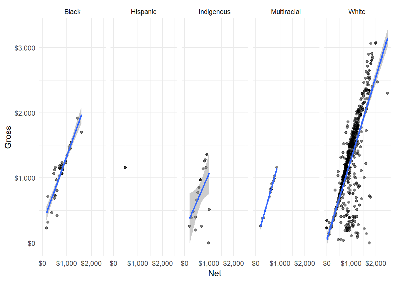
Modify facet_*() functions with arguments beyond the x ~ y formula.
- rows = accepts the number of rows in a facet grid
- cols = accepts the number of columns
- labeller = accepts new strip names
YOUR TURN: FACETING
Unfortunately, the R widget cannot visualize faceting (yet).
Open a new RStudio script. Copy and paste the below code.
Use a facet_*() function on variable cut.
1.5.7 The Themes Layer
The themes layer allows you to customize ever pixel of non-data ink in your plot.
- Function
themes()is the workhorse function for this layer themes()arguments are a large but consistent framework- Functions beginning with
theme_set premade themes - The themes layer adjusts every non-data pixel
Everything we’ve done so far, plus changing the facet strip labels:
ggplot(hancock,
       aes(x = net,
           y = gross)) +
  geom_point(alpha = 0.5,
             color = "grey30") +
  geom_smooth(alpha = 0.5,
              method = "lm") +
  theme_minimal() +
  scale_x_continuous(name = "Net",
                     breaks = pretty_breaks(3),
                     labels = dollar) +
  scale_y_continuous(name = "Gross",
                     breaks = pretty_breaks(3),
                     labels = dollar) +
  facet_wrap(facets = . ~ ethnicity) +
  theme(strip.text = element_text(face = "bold",
                                  color = "grey40",
                                  family = "Verdana"))   # The framework in action
So what the hell was that? There’s a whole consistent framework here!
There’s a few hierarchies of functions and arguments that we’ll look at below.
We’ve saved the above plot in object p, which we’ll use herein.
First Entering theme(): You’ll get hit with four short arguments:
- line = modifies all lines in the plot
- rect = modifies all rectangles in the plot
- text = modifies all text in the plot
- title = modifies just titles in the plot
p + theme(text = ...)Latter Arguments in theme(): More specific argument families for each element.
- axis arguments for axis lines, ticks, and text
- legend arguments for boxes, keys, spacing, text, and titles
- panel arguments for overall plot spacing and grid lines
- plot arguments for tags, titles, and margins
- strip arguments for facet strip text and backgrounds
p + theme(axis.title = ...)Once Argument is Selected: Arguments typically accept theme element functions:
- All element functions begin with
element_ element_rect()applies to rectangleselement_line()applies to lineselement_text()applies to textelement_blank()removes it
p + theme(axis.title = element_text(color = "gray50",
                                    face = "bold",
                                    size = 10))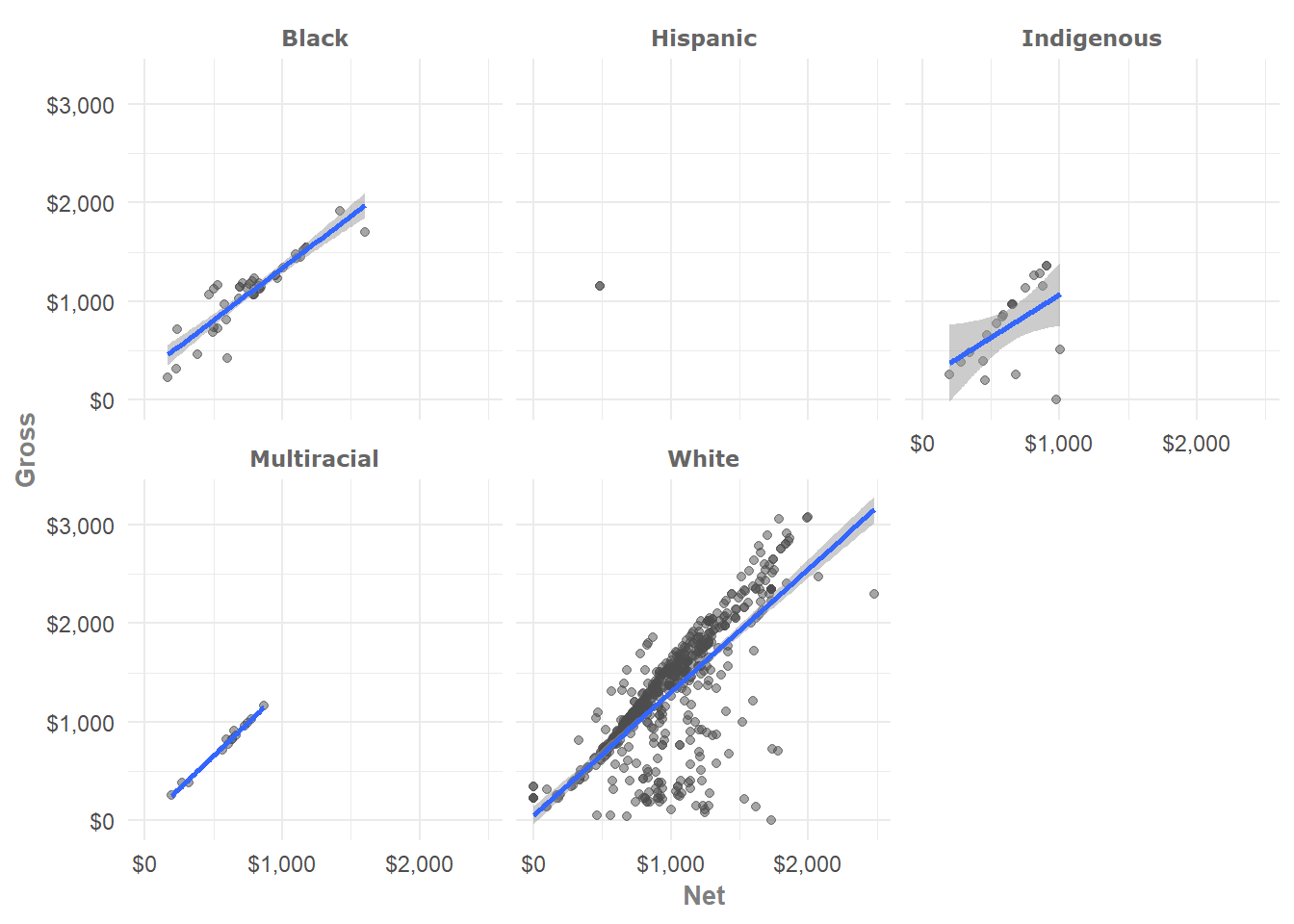
YOUR TURN: CUSTOMIZING TITLE THEMES
Load package scales to help format our scales. In themes():
- Change argument ‘x =’ in
labs()to “Year” - Format the plot’s axes title color to “grey20”
- Make the main title size 12 and “bold” face
- Continue experimenting with modifications
1.6 Interactive Charts with “plotly”
On a brief side note, you can make your “ggplot2” plots interactive with “plotly”.
Saving “ggplot” Objects: You can save plots as objects with assignment, or <-:
library(scales)
library(ggplot2)

p <- ggplot(hancock,              # Modified plot assigned to "p" with <-
       aes(x = net,
           y = gross)) +
  geom_point(alpha = 0.5,
             color = "grey30") +
  geom_smooth(alpha = 0.5,
              method = "lm") +
  theme_minimal() +
  scale_x_continuous(name = "Weekly Net",
                     labels = dollar,
                     breaks = pretty_breaks(3)) +
  scale_y_continuous(name = "Weekly Gross",
                     labels = dollar,
                     breaks = pretty_breaks(4)) +
  facet_wrap(facets = . ~ ethnicity)
Plotlify! Once loaded, use function ggplotly() on your ggplot oject:
library(plotly)

ggplotly(p)       # Insert your ggplot object!
Sweet. Not perfect - but with a bit of TLC it’d be right as rain.
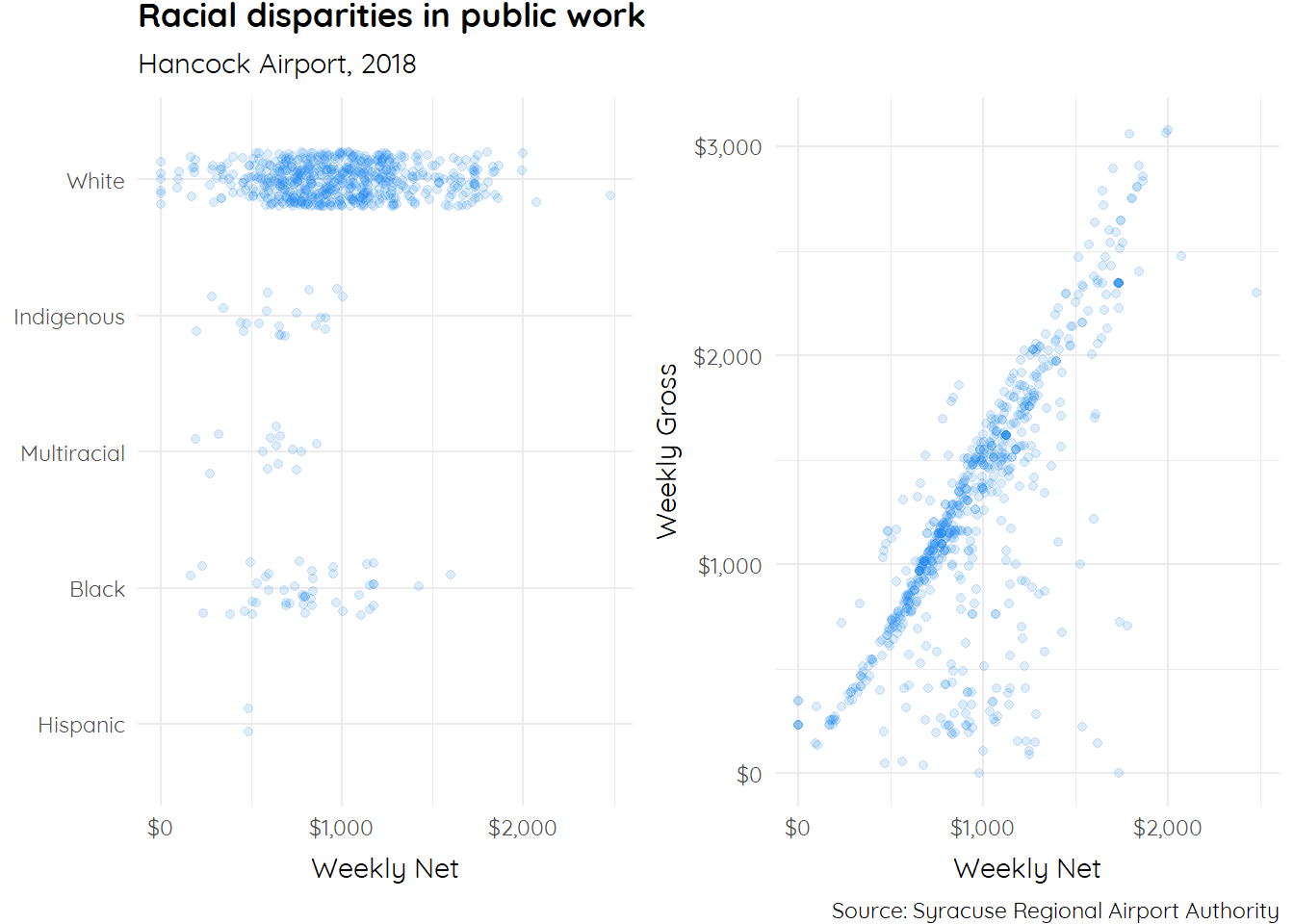
1.7 Combining Plots
Overlaying one plot ontop of another is simply a matter of adding geoms.
Needed within those geoms may be new calls to aes().
Let’s begin with a simple jitter plot of net distributed by ethnicity:
ggplot(hancock,
       aes(x = net,
           y = ethnicity)) +
  geom_jitter(height = 0.3,
              alpha = 0.3,
              color = "steelblue") +
  theme_minimal()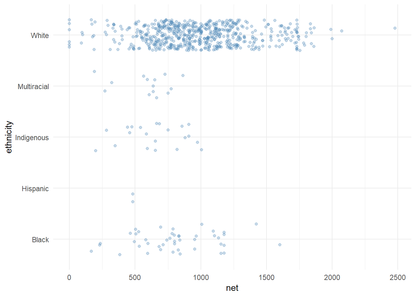
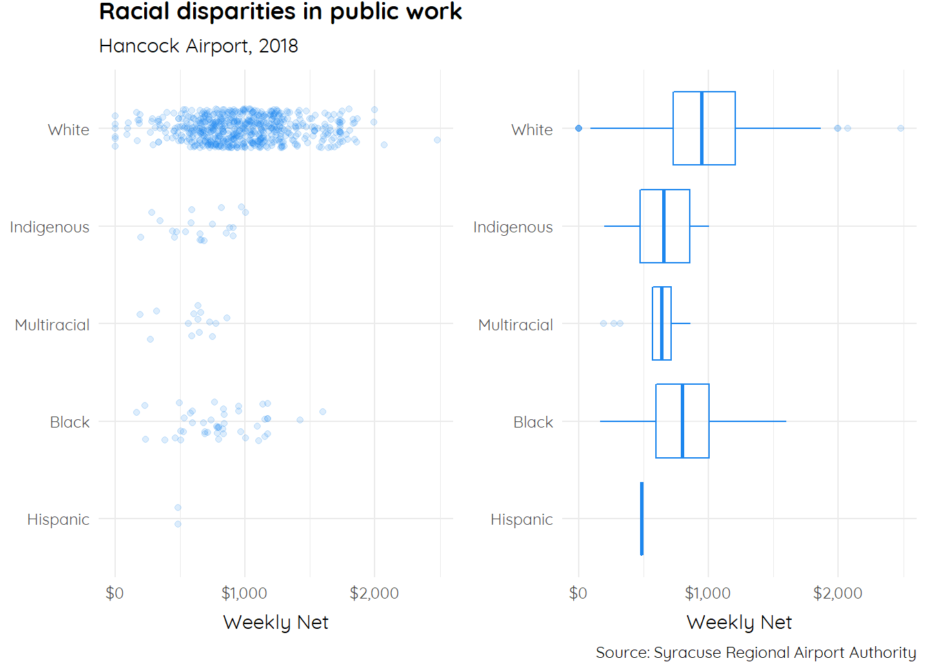
Overlay plots by adding additional geom. Here, we add geom_boxplot():
ggplot(hancock,
       aes(x = ethnicity,
           y = net)) +
  geom_jitter(height = 0.3,
              alpha = 0.3,
              color = "steelblue") +
  coord_flip() +
  theme_minimal() +
  geom_boxplot(height = 0.3,              # Simply add the new geom
               fill = "transparent",      # Modify attributes accordingly
               color = "grey50")
The Final Product: A plot overlay with some finishing touches:
library(extrafont)

ggplot(hancock,
       aes(x = reorder(ethnicity, net),
           y = net)) +
  geom_jitter(height = 0.3,
              alpha = 0.4,
              color = "dodgerblue") +
  coord_flip() +
  theme_minimal() +
  geom_boxplot(height = 0.2,
               fill = "transparent",
               color = "grey50") +
  labs(title = "Distribution of weekly net by ethnicity",
       subtitle = "Hancock Airport, 2018",
       x = NULL,
       y = "Weekly Net",
       caption = "Source: Syracuse Regional Airport Authority") +
  scale_y_continuous(labels = dollar) +
  theme(text = element_text(family = "Calibri Light"),
        axis.title.x = element_text(vjust = -1,
                                    color = "grey20"),
        plot.caption = element_text(vjust = -1,
                                    color = "grey60"),
        plot.subtitle = element_text(vjust = 1,
                                     color = "grey30"),
        plot.title = element_text(vjust = 2,
                                  color = "grey10"),
        axis.text.x = element_text(colour = "grey10"),
        axis.text.y = element_text(colour = "grey10"))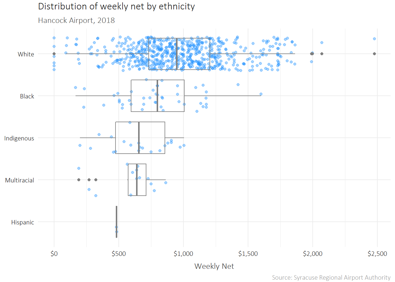
1.8 Package “ggplot2” Extensions
We used a “ggplot2” extension in the introduction to this chapter: “GGally”.
You can find a list of every single extension at the ggplot2 extensions gallery.
1.9 Further Resources
To review the practice data from Hancock Airport, get the raw data URL here.
There’s a lot to master here - but it’s worth it. These can help:
- ggplot2 Tidyverse Page
- ggplot2 Cheat Sheet (RStudio)
- ggplot2 Extensions Gallery
- The R Graph Gallery
- R Documentation: Scales
- R Graphing Library (Plotly)
- “Visualization with ggplot2: Part I”
- “Visualization with ggplot2: Part II”
- “Visualization with ggplot2: Part III”