1 Getting Data into R

1 Key Concepts

In this chapter, we’ll explore the following key concepts:

File Formats
RData Format
Flat or Text Files
Wrapper Functions

1 Key Takeaways

Too long; didn’t read? Here’s what you need to know:

Importing data is called “reading in” data in R, and done with read*() functions
Know as what format your data are stored to use the appropriate function
Read in statistical software files with packages “foreign” or “haven”
Read in JSON files with package “jsonlite”
Read directly from the web with URLs

1.1 “Reading In” Data

Importing data is also called reading in data in R.

Many base R functions begin with read, like read.csv() and read.table().

Some R packages have new reading functions, like read_csv() in the “readr” package.

Figure 1.1: Be careful with what you read into R!

Source: Perry Bible Fellowship

1.2 Know Thy Data: File Formats

"If you know the [data] and know yourself,

you need not fear the result of a hundred [analyses]."

Sun Tzu, The Art of [Data Science]

If you want to get certain data into R, you must know the file format.

File formats are standardized frameworks for encoding and storing information
Some file formats are better than others, depending on the information stored
Determine a file’s format by its filename extension, e.g. .csv
The most common data file formats include .csv, .tsv, and .xlsx

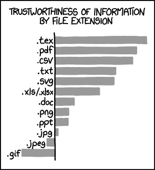
Figure 1.2: Certain formats are better for storing data.

Source: XKCD

1.2.1 Text or “Flat” Files

flatly /ˈflatli/

Showing little interest or emotion.

In a firm and unequivocal manner; absolutely.

In a smooth and even way.

Oxford English Dictionary

The far most familiar family of file formats includes text data or flat files.

Flat files are simple, standard formats that use plain text
Flat files are ubiquitous, non-proprietary, and accessible
Converting a spreadsheet into a text file will “flatten it”, removing all formatting

PRO TIP:

Flat files are ideal for sharing data with collaborators.

Not everyone has spreadsheet software, but anyone can use flat files
Flat files don’t preserve formats, like borders and highlighted cells
Flat files force users to store data tabularly “flatly”

Comma-separated values or CSV files store data in plain text:

Each line in a CSV file represents one row
Each value in a CSV file is separated by a comma
Therefore, each comma designates a separate column

A CSV in the Wild: Observe the following public construction records on GitHub:

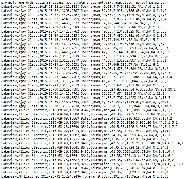
Figure 1.3: What can you decode by observing this raw CSV file?

A Wrangled CSV: R (and other software) interpret and tame these formats tabularly.

##     project       name     ending   zip  ssn      class hours rate  gross
## 1  Lakeview Ajay Glass 2015-08-02 14612 3888 Journeyman    40 18.5  740.0
## 2  Lakeview Ajay Glass 2015-08-02 13205 2807 Journeyman    32 28.7  918.4
## 3  Lakeview Ajay Glass 2015-08-02 14428 7762 Journeyman    40 33.7 1348.0
## 4  Lakeview Ajay Glass 2015-08-02 14549 9759 Journeyman    26 33.7  876.2
## 5  Lakeview Ajay Glass 2015-08-09 14433 5632 Journeyman    32 17.0  544.0
## 6  Lakeview Ajay Glass 2015-08-09 14612 3888 Journeyman    40 18.5  740.0
## 7  Lakeview Ajay Glass 2015-08-09 14428 7762 Journeyman    40 33.7 1348.0
## 8  Lakeview Ajay Glass 2015-08-09 13118 2838 Journeyman    16 28.7  459.2
## 9  Lakeview Ajay Glass 2015-08-16 14433 5632 Journeyman    32 17.0  544.0
## 10 Lakeview Ajay Glass 2015-08-16 14612 3888 Journeyman    42 18.5  795.5
##        net  sex race ot pdf_no pdf_pg pg_ob
## 1   511.31 <NA> <NA>  0      1      1     1
## 2   586.65 <NA> <NA>  0      1      1     2
## 3  1025.92 <NA> <NA>  0      1      1     3
## 4   891.08 <NA> <NA>  0      1      1     4
## 5   384.08 <NA> <NA>  0      1      3     1
## 6   657.86 <NA> <NA>  0      1      3     2
## 7  1025.92 <NA> <NA>  0      1      3     3
## 8   361.98 <NA> <NA>  0      1      3     4
## 9   384.08 <NA> <NA>  0      1      5     1
## 10  616.28 <NA> <NA>  0      1      5     2

Tab-separated values or TSV files store data in plain text:

Like CSV, each line in a TSV file represents one row
Also like CSV, each value in a CSV file is separated by a tab
Each tab designates a separate column

A TSV in the Wild: Observe the same public construction records on GitHub:

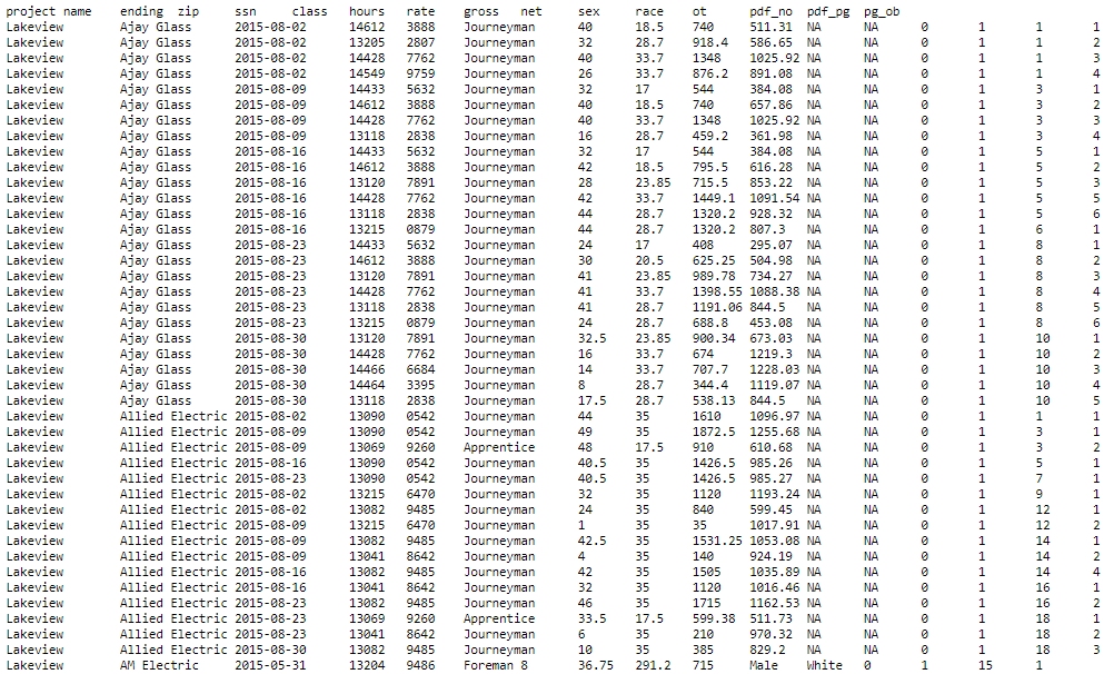
Figure 1.4: Raw TSV files are much more intepretable thanks to tabulation.

1.2.2 Excel File Formats

Microsoft Excel files are significantly different from text or flat files.

All Excel file extensions begin with .xls; a workbook is in .xlsx format
Excel workbooks with multiple sheets must be read in one sheet at a time
Multiple packages can help R handle Excel files, e.g. readxl, XLConnect, gdata

WARNING:

Reading Excel files into R will remove all formatting, like:

Highlighted and color-coded cells
Font formatting, e.g. bold and italics
Borders, merged cells, formulas, and macros

Some Excel users use formatting to represent information. For example, a user may use red, yellow, and green to represent a categorical variable like “low”, “medium”, and “high”, respectively. In such cases, create a new column to store these data.

Excel Files in the Wild: It’s common to see Excel files with heavy formatting:

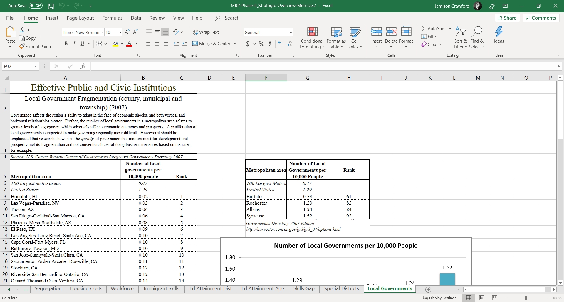
Figure 1.5: If R were to import this file, as is, what information would survive?

Source: Special District Governments, CNY Vitals Legacy

1.2.3 JSON File Format

The JSON format stands for “JavaScript Object Notation”:

JSON files use extension .json
Like TSV files, JSON files are concise and well-structured
Also like TSV, JSON files are generally human-readable
JSON structure differs across files and are read into R differently
Packages like jsonlite help R read in .json files

JSON Files in the Wild: Check out these Game of Thrones subtitles in JSON format:

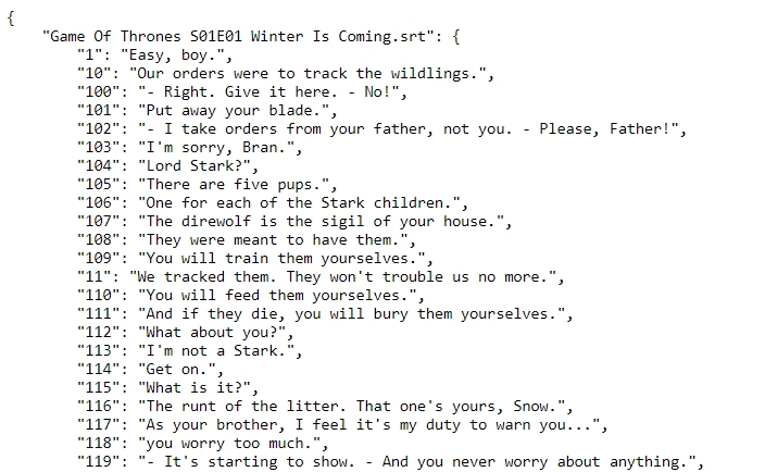
Figure 1.6: This JSON file has nested arrays, or sets of values within sets of values.

1.2.4 Statistical Software Formats

Each major statistical software has its own (sometimes proprietary) file format, e.g.:

SPSS uses extensions .sav and .por
SAS uses extensions .sas7bdat and .sas7bcat
STATA uses extension .dta

Different packages exist for importing statistical software files, e.g.:

Package foreign, created by R’s core team, supports many formats
Package haven, created by Hadley Wickham, is faster but for fewer formats

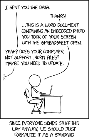
Figure 1.7: .NORM files do not exist.

Source: XKCD

1.2.5 RData Format

You may have noticed, when working in R, that you’re asked to save your workspace.

When saving a workspace, .rdata or .rda files are stored in the working directory.

You can manually save part or all of your workspace with function save()
You can then load part or all of your workspace with function load()
.rdata and .rda files store your session’s objects, command history, etc.
If creating an object is computationally expensive, consider saving it!

1.2.6 Conclusions

There are a variety of file formats that you can read into R.

For virtually every file format, there are functions and packages to import them.

You must know the file’s format to decide on the best import function.

1.3 Key Functions for Importing Data

Once you’ve identified the extension type, you should consider how to read it into R.

Is it a flat or text file?
What character delimits each value, e.g. ,, ;?
Can you read it in using base R or do you need a new package?
What other arguments should you specify to ensure success?

We’ll look at a few common functions for importing common formats.

1.3.1 Workhorses & Wrapper Functions:

The workhorse of all base R reading functions is read.table().

Thanks to its modifiability, function read.table() is remarkably flexible.

Not only does it import most file types, it’s used by many wrapper functions.

QUESTION

You can see whats under a function’s hood by typing it without ().

Look at the internals of function read.csv(). What function is used?

read.csv

## function (file, header = TRUE, sep = ",", quote = "\"", dec = ".", 
##     fill = TRUE, comment.char = "", ...) 
## read.table(file = file, header = header, sep = sep, quote = quote, 
##     dec = dec, fill = fill, comment.char = comment.char, ...)
## <bytecode: 0x00000000132bda28>
## <environment: namespace:utils>

A wrapper function is a modified version of a more powerful and versatile function.

Each is optimized for a specific task, like read.csv() - a very common function.

Wrapper functions are like customized tools. Their toolboxes are packages.

1.4 Base R: Reading CSV Files

Reading comma-separated values (CSV) files is done with base R’s read.csv() function.

Only requires one argument: path =
Argument path = accepts the directory path or a web URL

read.csv(file = "~/dp4ss-textbook/my_data.csv")
read.csv(file = "http://www.ds4ps.com/textbook/my_data.csv")

We can read in Syracuse, NY lead violations directly from the city’s open data portal.

  #' Put your URL in quotes; here, we name it "url"
  #' Use function paste0() to join long strings of text

url <- paste0("https://opendata.arcgis.com/datasets/", 
              "c15a39a8a00e48b1a60c826c8a2cb3e0_0.csv")

lead_data <- read.csv(file = url,                  # Use object storing URL text
                      stringsAsFactors = FALSE)    # Always include this argument!

Now, we have a locally-stored dataset:

lead_data[1:10, 1:4]      # Bracks specify rows and columns to include

Consider the following notable arguments for read.csv():

file = takes a string of text, either a directory and file name or a URL
nrow = take a number, setting the limit of rows to read in
stringsAsFactors = converts text into categories (not cool!)
col.names = takes an array made with c() to rename variables
colClasses = also takes an array using c() to specify classes

PRO TIP: READING FROM CLIPBOARDS

Why not read the data you’ve copied to your clipboard?

In this approach, just change the first argument, file =, to “clipboard”.

read.csv(file = "clipboard")

1.5 Base R: Reading TSV & Other Delimited Formats

There are many ways to delimit data in a flat (text) file.

For example, tab-delimited, semicolon-delimited, asterisk-delimited - you get it.

In these instances, you can use function read.delim() to specify the delimiter.

Here, we specify the delimiter as a comma, ,:

lead <- read.delim(file = url, 
                   stringsAsFactors = FALSE,
                   sep = ',')                   # Specifies delimiter

You can specify your delimiter as any character you wish:

read.delim(file = my_file, sep = ',')
read.delim(file = my_file, sep = ';')
read.delim(file = my_file, sep = '\t')          # Tab-delimited

You can also read in any flat file, point-and-click, with RStudio’s import wizard:

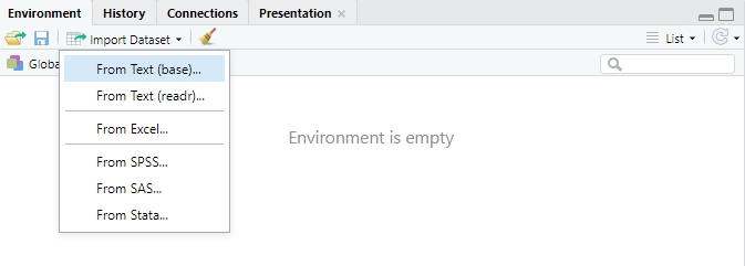
Figure 1.8: Open the import wizard in the Environment pane.

In the import wizard, you can specify arguments with a user-friendly interface.

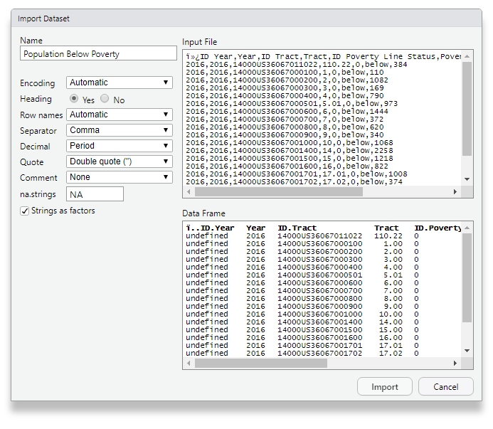
Figure 1.9: Click your way to victory!

1.6 Package “readr” Functions

The “readr” package improves on several functions in base R’s reading toolkit, e.g.:

Built into RStudio
All functions begin with read_
All functions have more consistent argument names
Automatically sets stringsAsFactors = to FALSE
Expanded, specialized functions for specific data types
Enhances your data frame by converting it into a “tibble”

Observe the output from the “tibble” data frame. What’s different?

library(readr)

url <- paste0("https://opendata.arcgis.com/datasets/", 
              "c15a39a8a00e48b1a60c826c8a2cb3e0_0.csv")

read_csv(url)

PRO TIP

Consider getting used to tibbles (enhanced data frames from “readr”).

Tibbles print a lot more details about your data, e.g. variable classes
They cooperate more easily with packages in the Rstudio ecosystem
Also, they automatically truncate output to appear more organized

ANOTHER PRO TIP

You can change variable classes much more easily in “readr” functions.

Short string representation allows you to specify classes with one character:

“c” for character
“d” for double
“i” for integer
“l” for logical
"_" to exclude variable

In a function, to specify 3 logical, 2 integer, and 4 character variables:

read_csv(path = path, col_types = c("llliicccc"))

1.7 Importing Excel Files

There are many packages available for reading in Excel’s .xlsx format.

Package “readxl” is part of the same package ecosystem as “readr”.

Allows new Excel-related functions, like read_xlsx()
Lists all sheets in a workbook with excel_sheets()
Specify certain sheets with argument sheet =

library(readxl)

read_xlsx(path = url, 
          sheet = "FY 2018 Revenue",    # Specify sheet
          range = "B3:G78",             # Specify range
          trim_ws = TRUE,               # Remove leading/trailing spaces
          col_types = "dcic_cli_cc")    # Specify variable classes

Of course, RStudio has macros set up if you’d prefer:

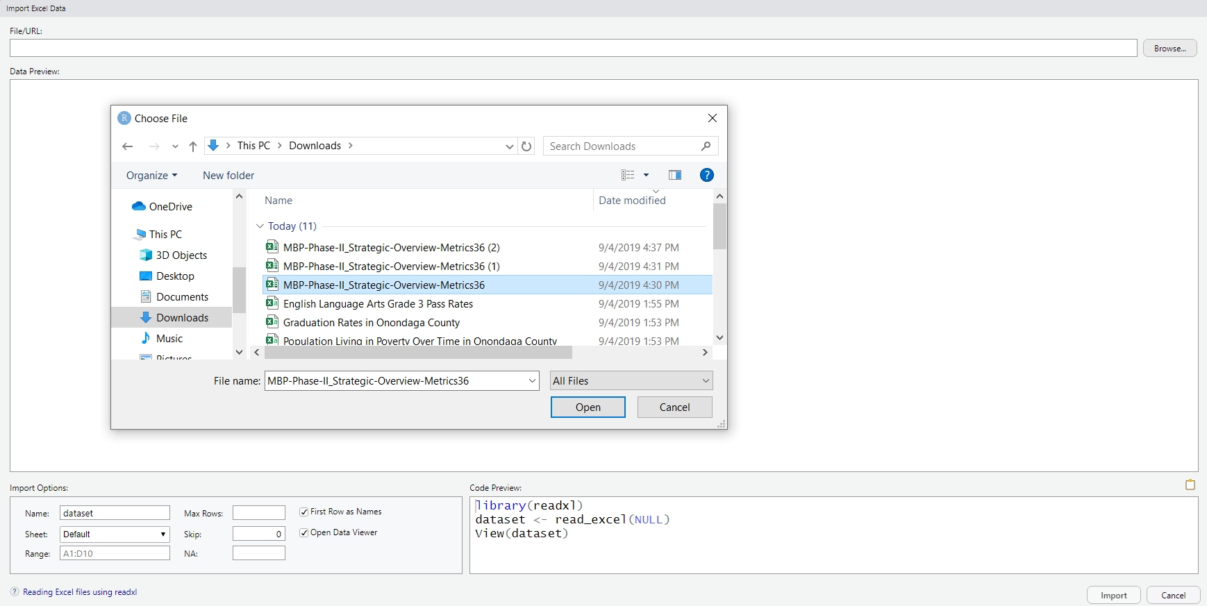
Figure 1.10: RStudio’s wizard for importing from Excel.

Figure 1.11: Excel at times.

Source: Reddit

LIFE HACK

Using RStudio’s import wizard may seem like such a noob move.

It is, but that doesn’t mean you can’t turn it into a clutch move.

Even when using wizards and macros, code will still run in the R console:

Copy that code and throw it into your script. It’s often faster than typing.

1.8 Importing Statistical Software Files

Two packages are commonly used to import files from SPSS, SAS, STATA and other software:

Package “foreign” was developed by the R core team and highly versatile
Package “haven” was developed by RStudio and only reads in SPSS, SAS, and STATA

Their differences are similar to those between base R and “readr” functions.

read.dta() is equivalent to read_dta() in the packages, respectively
read.spss() is equivalent to read_spss(), respectively
read.stata() is equavalent to read_stata(), and so on

1.9 Getting Data Off of the Web

There are a variety of methods to get data out of the web and into R.

Here are a few popular methods:

1.9.1 Retrieve Download URLs

Many times, it’s a matter of copying URLs from links that download datasets.

Here, we find the “Download” button on a City Of Pheonix Open Data dataset:

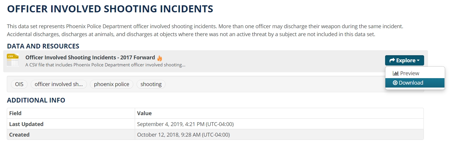
Figure 1.12: Open data portals make it easy to download data straight into R.

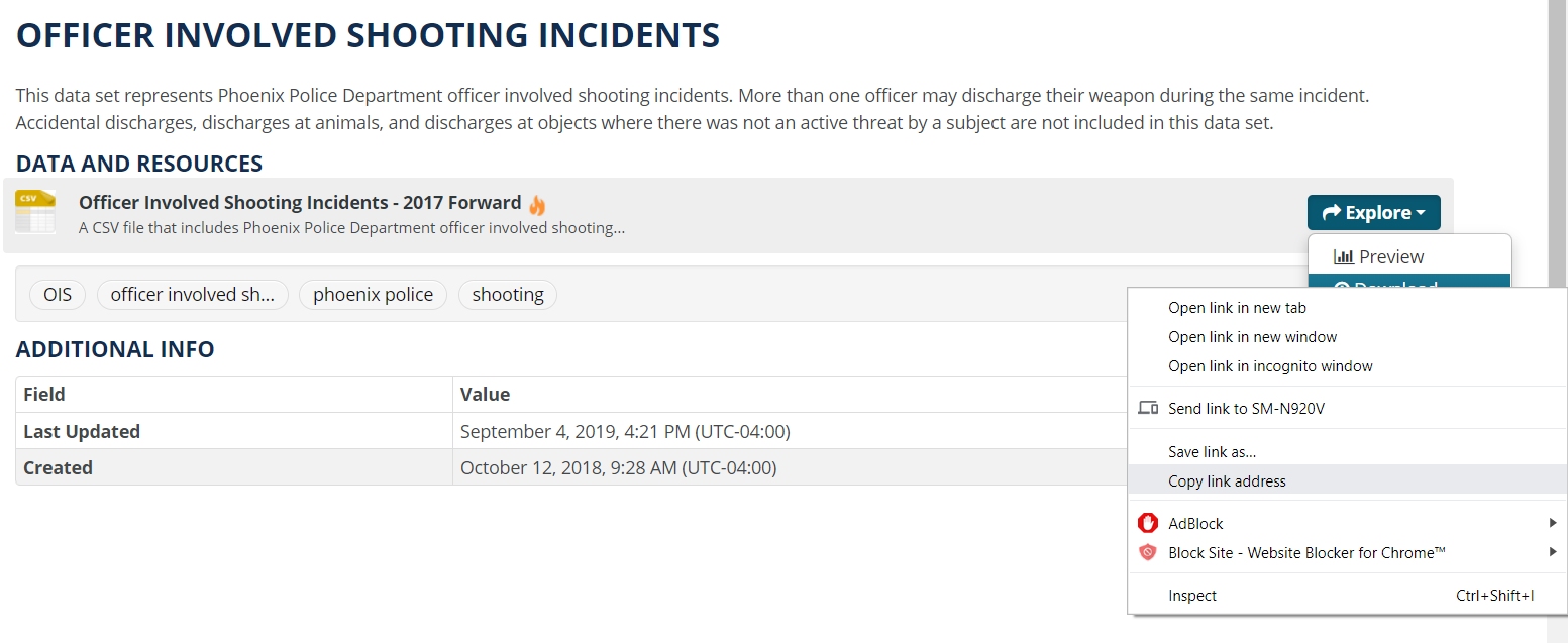
Figure 1.13: Right-click “Download” to copy the URL.

You can save the URL in an object or use the whole string for the path = argument.

1.9.2 Retrieve Raw Data URLs

GitHub is riddled with datasets.

You can often find a “Download” button for them.

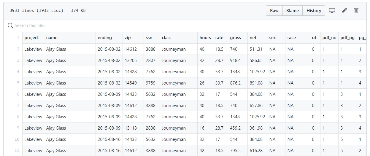
Figure 1.14: The head of a table in GitHub’s data viewer.

In the event that you cannot find a “Download” button, click on “Raw”.

You can use the URL provided to read the data into R.

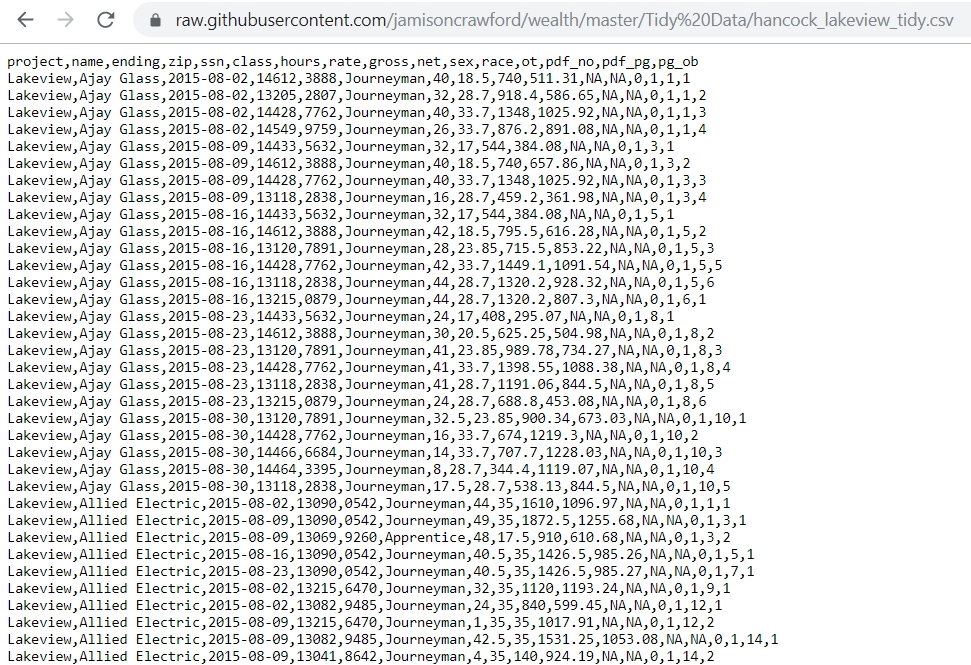
Figure 1.15: The raw CSV file, with the URL for reading into R.

1.10 Further Resources

The following resources should help you further your knowledge on reading in data.