1 Introduction to R

This lecture introduces you to basic operations when you first start using R such as navigation, the object-oriented framework, loading a package, and creating some data vectors.

1.1 Navigation

You need to know a few operations to help you maneuver the R work environment, such as listing objects (datasets and functions) that are active, changing your working directory, listing available files, and finding help.

1.1.1 Setting Your Working Directory

When you are ready to load data, R needs to know where to look for your files. You can check what is avaiable in the current directory (i.e. folder) by asking to list all of the current files using dir().

dir()

If the file that you need is located in a different folder, you can change directories easily in R Studio by Session -> Set working director -> Choose directory (or Ctrl + Shift + H).

If you are writing a script, you want to keep track of this step so that it can be reproduced. Use the function get.wd() to check your current working directory, and set.wd() to change. You need to specify your path as an argument to this function, such as.

setwd( "C:/user/projects/financial model" )

NOTE! R uses unix style notation with forward slashes, so if you copy and paste from Windows it will look like this, with back slashes:

setwd( "C:\user\projects\financial model" )

You will need to change them around for it to work.

It is best to save all of your steps in your scripts so that the analysis can be reproduced by yourself or others. In some cases you are doing exploratory or summary work, and you may want to find a file a quickly. You can use the file.choose() function to open a GUI to select your file directly. This function is used as an argument inside of a load data function.

my.dat <- read.csv( file.choose() )

1.2 Commenting Code

Most computer languages have a special character that is used to “comment out” lines so that it is not run by the program. It is used for two important purposes. First, we can add text to document our functions and it will not interfere with the program. And two, we can use it to run a program while ignoring some of the code, often for debugging purposes.

The # hash tag is used for comments in R.

##==============================================
##
##  Here is some documentation for this script
##
##==============================================

x <- 1:10

sum( x )

## [1] 55

# y <- 1:25     # not run

# sum( y )      # not run

1.3 Help

You will use the help functions frequently to figure out what arguments and values are needed for specific functions. Because R is very customizable, you will find that many functions have several or dozens of arguments, and it is difficult to remember the correct syntax and values. But don’t worry, to look them up all you need is the function name and a call for help:

help( dotchart ) # opens an external helpfile

If you just need to remind yourself which arguments are defined in a function, you can use the args() command:

args( dotchart )

## function (x, labels = NULL, groups = NULL, gdata = NULL, offset = 1/8, 
##     ann = par("ann"), xaxt = par("xaxt"), frame.plot = TRUE, 
##     log = "", cex = par("cex"), pt.cex = cex, pch = 21, gpch = 21, 
##     bg = par("bg"), color = par("fg"), gcolor = par("fg"), lcolor = "gray", 
##     xlim = range(x[is.finite(x)]), main = NULL, xlab = NULL, 
##     ylab = NULL, ...) 
## NULL

If you can’t recall a function name, you can list all of the functions from a specific package as follows:

help( package=“stats” ) # lists all functions in stats package

1.4 Install Programs (packages)

When you open R by default it will launch a core set of programs, called “packages” in R speak, that are use for most data operations. To see which packages are currently active use the search() function.

search()

## [1] ".GlobalEnv"        "package:stats"     "package:graphics" 
## [4] "package:grDevices" "package:utils"     "package:datasets" 
## [7] "package:methods"   "Autoloads"         "package:base"

These programs manage the basic data operations, run the core graphics engine, and give you basic statistical methods.

The real magic for R comes from the over 7,000 contributed packages available on the CRAN: https://cran.r-project.org/web/views/

A package consists of custom functions and datasets that are generated by users. They are packaged together so that they can be shared with others. A package also includes documentation that describes each function, defines all of the arguments, and documents any datasets that are included.

If you know a package name, it is easy to install. In R Studio you can select Tools -> Install Packages and a list of available packages will be generated. But it is easier to use the install.packages() command. We will use the Lahman Package in this course, so let’s install that now.

Description This package provides the tables from Sean Lahman’s Baseball Database as a set of R data.frames. It uses the data on pitching, hitting and fielding performance and other tables from 1871 through 2013, as recorded in the 2014 version of the database.

See the documentation here: https://cran.r-project.org/web/packages/Lahman/Lahman.pdf

install.packages( "Lahman" )

You will be asked to select a “mirror”. In R speak this just means the server from which you will download the package (choose anything nearby). R is a community of developers and universities that create code and maintain the infrastructure. A couple of dozen universities around the world host servers that contain copies of the R packages so that they can be easily accessed everywhere.

If the package is successfully installed you will get a message similar to this:

package ‘Lahman’ successfully unpacked and MD5 sums checked

Once a new program is installed you can now open (“load” in R speak) the package using the library() command:

library( "Lahman" )

If you now type search() you can see that Lahman has been added to the list of active programs. We can now access all of the functions and data that are available in the Lahman package.

1.5 Accessing Built-In Datasets in R

One nice feature of R is that is comes with a bunch of built-in datasets that have been contributed by users are are loaded automatically. You can see the list of available datasets by typing:

data()

This will list all of the default datasets in core R packages. If you want to see all of the datasets available in installed packages as well use:

data( package = .packages(all.available = TRUE) )

1.5.1 Basic Data Operations

Let’s ignore the underlying data structure right now and look at some ways that we might interact with data.

We will use the USArrests dataset available in the core files.

To access the data we need to load it into working memory. Anything that is active in R will be listed in the environment, which you can check using the ls() command. We will load the dataset using the data() command.

remove( list=ls() )

ls() # nothing currently available

## character(0)

data( "USArrests" )

ls() # data is now avaible for use

## [1] "USArrests"

Now that we have loaded a dataset, we can start to access the variables and analyze relationships. Let’s get to know our dataset.

names( USArrests )  # what variables are in the dataset?

## [1] "Murder"   "Assault"  "UrbanPop" "Rape"

nrow( USArrests )   # how many observations are there?

## [1] 50

dim( USArrests )    # a quick way to see rows and columns - the dimensions of the dataset

## [1] 50  4

row.names( head( USArrests ) )   # what are the obsevations (rows) in our data

## [1] "Alabama"    "Alaska"     "Arizona"    "Arkansas"   "California"
## [6] "Colorado"

summary( USArrests )   # summary statistics of variables

##      Murder          Assault         UrbanPop          Rape      
##  Min.   : 0.800   Min.   : 45.0   Min.   :32.00   Min.   : 7.30  
##  1st Qu.: 4.075   1st Qu.:109.0   1st Qu.:54.50   1st Qu.:15.07  
##  Median : 7.250   Median :159.0   Median :66.00   Median :20.10  
##  Mean   : 7.788   Mean   :170.8   Mean   :65.54   Mean   :21.23  
##  3rd Qu.:11.250   3rd Qu.:249.0   3rd Qu.:77.75   3rd Qu.:26.18  
##  Max.   :17.400   Max.   :337.0   Max.   :91.00   Max.   :46.00

We can see that the dataset consists of four variables: Murder, Assault, UrbanPop, and Rape. We also see that our unit of analysis is the state. But where does the data come from, and how are these variables measured?

To see the documentation for a specific dataset you will need to use the help() function:

help( "USArrests" )

We get valuable information about the source and metrics:

Description This data set contains statistics, in arrests per 100,000 residents for assault, murder, and rape in each of the 50 US states in 1973. Also given is the percent of the population living in urban areas.

Format A data frame with 50 observations on 4 variables.

Murder: numeric Murder arrests (per 100,000)
Assault: numeric Assault arrests (per 100,000)
UrbanPop: numeric Percent urban population
Rape: numeric Rape arrests (per 100,000)

To access a specific variable inside of a dataset, you will use the $ operator between the dataset name and the variable name:

summary( USArrests$Murder )

##    Min. 1st Qu.  Median    Mean 3rd Qu.    Max. 
##   0.800   4.075   7.250   7.788  11.250  17.400

summary( USArrests$Assault )

##    Min. 1st Qu.  Median    Mean 3rd Qu.    Max. 
##    45.0   109.0   159.0   170.8   249.0   337.0

# Is there a relationship between urban density and crime?

plot( USArrests$UrbanPop, USArrests$Murder, 
      frame.plot=F, pch=19, col="gray" )
abline( lm( USArrests$Murder ~ USArrests$UrbanPop ), col="red" )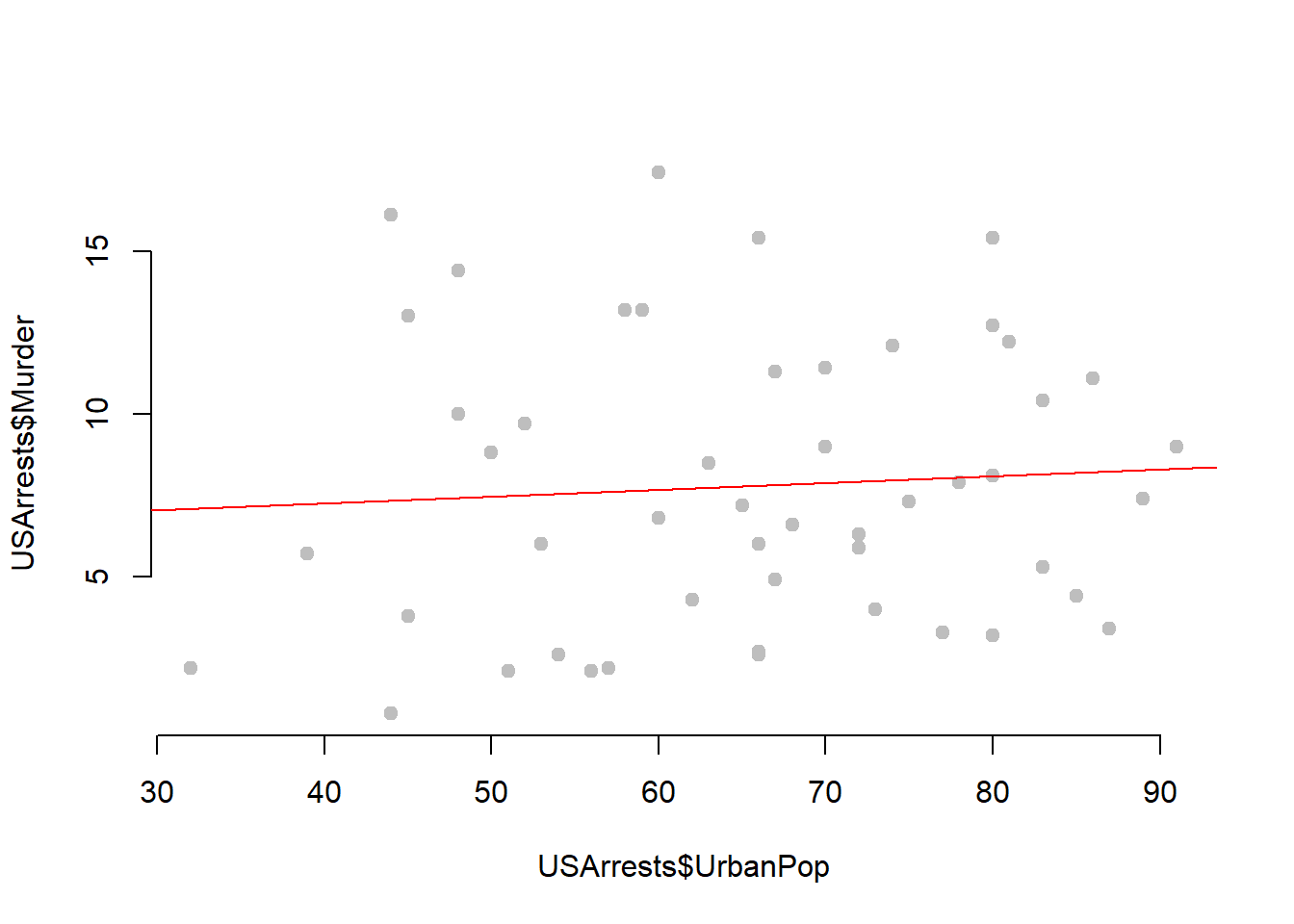

1.5.2 Using the Lahman Data

Let’s take a look at some of the data available in the Lahman package.

data( package = "Lahman" ) # All datasets in package "Lahman":

TABLE NAME	DEFITION
AllstarFull	AllstarFull table
Appearances	Appearances table
AwardsManagers	AwardsManagers table
AwardsPlayers	AwardsPlayers table
AwardsShareManagers	AwardsShareManagers table
AwardsSharePlayers	AwardsSharePlayers table
Batting	Batting table
BattingPost	BattingPost table
CollegePlaying	CollegePlaying table
Fielding	Fielding table
FieldingOF	FieldingOF table
FieldingPost	FieldingPost data
HallOfFame	Hall of Fame Voting Data
LahmanData	Lahman Datasets
Managers	Managers table
ManagersHalf	ManagersHalf table
Master	Master table
Pitching	Pitching table
PitchingPost	PitchingPost table
Salaries	Salaries table
Schools	Schools table
SeriesPost	SeriesPost table
Teams	Teams table
TeamsFranchises	TeamFranchises table
TeamsHalf	TeamsHalf table
battingLabels	Variable Labels
fieldingLabels	Variable Labels
pitchingLabels	Variable Labels

We see that we have lots of datasets to choose from here. I will use the Master dataset, which is a list of all of the Major League Baseball players over the past century, and their personal information.

library( Lahman )    # loads Lahman package
data( Master )
head( Master )

Here are some common functions for exploring datasets:

names( Master )      # variable names
nrow( Master )       # 18,354 players included
summary( Master )    # descriptive statistics of variables

We can use help(Master) to get information about the dataset, including a data dictionary.

help( Master )

MASTER TABLE

Description

Master table - Player names, DOB, and biographical info. This file is to be used to get details about players listed in the Batting, Pitching, and other files where players are identified only by playerID.

Usage

data(Master)

Format

A data frame with 19105 observations on the following 26 variables.

playerID: A unique code asssigned to each player. The playerID links the data in this file with records on players in the other files.
birthYear: Year player was born
birthMonth: Month player was born
birthDay: Day player was born
birthCountry: Country where player was born
birthState: State where player was born
birthCity: City where player was born
deathYear: Year player died
deathMonth: Month player died
deathDay: Day player died
deathCountry: Country where player died
deathState: State where player died
deathCity: City where player died
nameFirst: Player’s first name
nameLast: Player’s last name
nameGiven: Player’s given name (typically first and middle)
weight: Player’s weight in pounds
height: Player’s height in inches
bats: a factor: Player’s batting hand (left (L), right (R), or both (B))
throws: a factor: Player’s throwing hand (left(L) or right(R))
debut: Date that player made first major league appearance
finalGame: Date that player made first major league appearance (blank if still active)
retroID: ID used by retrosheet, http://www.retrosheet.org/
bbrefID: ID used by Baseball Reference website, http://www.baseball-reference.com/
birthDate: Player’s birthdate, in as.Date format
deathDate: Player’s deathdate, in as.Date format

Details

debut, finalGame were converted from character strings with as.Date.

Source

Lahman, S. (2016) Lahman’s Baseball Database, 1871-2015, 2015 version, http://www.seanlahman.com/baseball-archive/statistics/

tab <- prop.table( table( Master$birthMonth ) )
names(tab) <- c("Jan","Feb","Mar","Apr","May","Jun","Jul","Aug","Sep","Oct","Nov","Dec")
dotchart( tab, pch=19, 
          xlab = "Proportion of MLB Players", 
          ylab = "Birth Month" )